Hands-On Machine Learning with Scikit-Learn & TensorFlow
Hands-On Machine Learning with Scikit-Learn and TensorFlow
Concepts, Tools, and Techniques to Build Intelligent Systemsby
Aurélien Géron
Preface
Actual production-ready Python frameworks:- Scikit-Learn is very easy to use, yet it implements many Machine Learning algorithms efficiently, so it makes for a great entry point to learn Machine Learning. Scikit Learn is a general machine learning library built on top of NumPy. It features a lot of utilities for general pre and post-processing of data. It is a library in Python used to construct traditional models.
- TensorFlow is a more complex library for distributed numerical computation using data flow graphs. It makes it possible to train and run very large neural networks efficiently by distributing the computations across potentially thousands of multi-GPU servers. TensorFlow was created at Google and supports many of their large-scale Machine Learning applications. It was open-sourced in November 2015.
1. The Machine Learning Landscape
What Is Machine Learning?
Why Use Machine Learning?
Types of Machine Learning Systems
Supervised/Unsupervised Learning
In supervised learning, the training data you feed to the algorithm includes the desired solutions, called labels.
Given a set of features, the task to predict a target numeric value is called the predictor.
To train the system, you need to give it many example cases, including both their predictors and their labels
The methods used to analyze correlations between variables are called regression.
In unsupervised learning, the training data is unlabeled. The system tries to learn without a teacher.
Some algorithms can deal with partially labeled training data, usually a lot of un-labeled data and a little bit of labeled data. This is called semisupervised learning.
Reinforcement Learning is a very different beast. The learning system, called an agent in this context, can observe the environment, select and perform actions, and get rewards in return.
It must then learn by itself what is the best strategy, called a policy, to get the most reward over time. A policy defines what action the agent should choose when it is in a given situation.
Batch and Online Learning
Another criterion used to classify Machine Learning systems is whether or not the system can learn incrementally from a stream of incoming data.In batch learning, the system is incapable of learning incrementally: it must be trained using all the available data.
First the system is trained, and then it is launched into production and runs without learning anymore; it just applies what it has learned. This is called offline learning.
In online learning, you train the system incrementally by feeding it data instances sequentially, either individually or by small groups called mini-batches.
Instance-Based Versus Model-Based Learning
The instance-based learning learns the examples by heart, then generalizes to new cases using a similarity measure.
For ex., the spam filtering system would flag an email as spam if it has many words in common with a known spam email(instance).
The model-based learning uses a model built from known instances then use that model to make predictions.
You need to specify a performance measure and either define a utility function (or fitness function) that measures how good your model is, or you can define a cost function that measures how bad it is.
For linear regression problems, people typically use a cost function that measures the distance between the linear model’s predictions and the training examples; the objective is to minimize this distance.
This is where the Linear Regression algorithm comes in: you feed it your training examples and it finds the parameters that make the linear model fit best to your data. This is called training the model.
Main Challenges of Machine Learning
Insufficient Quantity of Training Data
Nonrepresentative Training Data
Poor-Quality Data
Irrelevant Features
Overfitting the Training Data
overfitting: it means that the model performs well on the training data, but it does not generalize well.
Underfitting the Training Data
Stepping Back
Testing and Validating
The only way to know how well a model will generalize to new cases is to actually try it out on new cases.
2. End-to-End Machine Learning Project
Working with Real Data
It is best to actually experiment with real-world data, not just artificial datasets.In this chapter we chose the California Housing Prices dataset from the StatLib repository.
Look at the Big Picture
The California census data. This data has metrics such as the population, median income, median housing price, and so on for each block group in California.Frame the Problem
How does the company expect to use and benefit from this model?
This model’s output (a prediction of a district’s median housing price) will be fed to another Machine Learning system , along with many other signals. This downstream system will determine whether it is worth investing in a given area or not.
A sequence of data processing components is called a data pipeline.
Components typically run asynchronously. Each component pulls in a large amount of data, processes it, and spits out the result in another data store, and then some time later the next component in the pipeline pulls this data and spits out its own output, and so on.
Select a Performance Measure
A typical performance measure for regression problems is the Root Mean Square Error (RMSE). It measures the standard deviation4 of the errors the system makes in its predictions
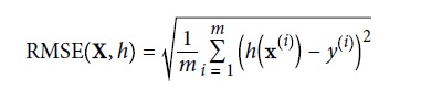
where:
- m is the number of instances in the dataset you are measuring the RMSE on.
- x(i) is a vector of all the feature values (excluding the label) of the i-th instance in the dataset. For ex., a district housing can be featured by: longitude, latitude, the number of inhabitants and a median income of the inhabitants.
- y(i) is its label (the desired output value for that instance). For ex., the the median house value of a district.
- X is a matrix containing all the feature values (excluding labels) of all instances in the dataset. There is one row per instance.
- h is your system’s prediction function, also called a hypothesis. When your system is given an instance’s feature vector x(i), it outputs a predicted value ŷ(i) = h(x(i)) for that instance.
- RMSE(X,h) is the cost function measured on the set of examples using your hypothesis h.
Check the Assumptions
Get the Data
Create the Workspace
$ export ML_PATH="$HOME/ml" # You can change the path if you prefer
$ mkdir -p $ML_PATH
$ pip3 install --upgrade jupyter matplotlib numpy pandas scipy scikit-learn
conda install jupyter matplotlib numpy pandas scipy scikit-learn
The Jupyter Notebook is an open-source web application that allows you to create and share documents that contain live code, equations, visualizations and narrative text. Uses include: data cleaning and transformation, numerical simulation, statistical modeling, data visualization, machine learning, and much more.
Now you can fire up Jupyter by typing:
jupyter notebook
A Jupyter server is now running in your terminal, listening to port 8888. You can visit this server by opening your web browser to http://localhost:8888/ (this usually happens automatically when the server starts).
You can create a new Python notebook by clicking on the "New" button on the Web. This does three things:
- it creates a new notebook file called Untitled.ipynb in your workspace You can rename this notebook by clicking "Untitled" and typing the new name.
- it starts a Jupyter Python kernel to run this notebook
- it opens this notebook in a new tab
Download the Data
import os
import tarfile
from six.moves import urllib

DOWNLOAD_ROOT = "https://raw.githubusercontent.com/ageron/handson-ml/master/"
HOUSING_PATH = "datasets/housing"
HOUSING_URL = DOWNLOAD_ROOT + HOUSING_PATH + "/housing.tgz"

def fetch_housing_data(housing_url=HOUSING_URL, housing_path=HOUSING_PATH):
    if not os.path.isdir(housing_path):
        os.makedirs(housing_path)
    tgz_path = os.path.join(housing_path, "housing.tgz")
    urllib.request.urlretrieve(housing_url, tgz_path)
    housing_tgz = tarfile.open(tgz_path)
    housing_tgz.extractall(path=housing_path)
    housing_tgz.close()

import pandas as pd

def load_housing_data(housing_path=HOUSING_PATH):
    csv_path = os.path.join(housing_path, "housing.csv")
    return pd.read_csv(csv_path)
Take a Quick Look at the Data Structure
Let's download the data and load the data using Pandas.
fetch_housing_data()
housing = load_housing_data()
housing.head()
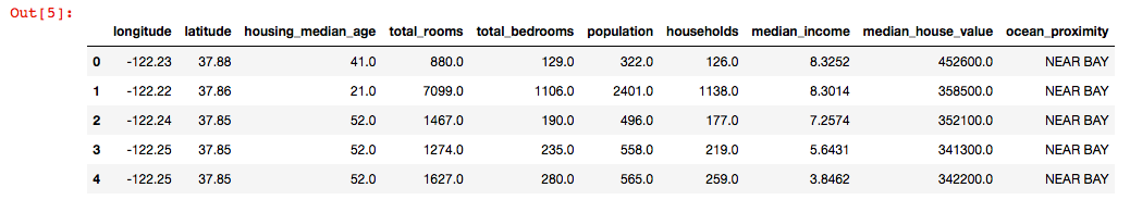
The info() method is useful to get a quick description of the data, in particular the total number of rows, and each attribute’s type and number of non-null values
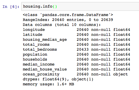
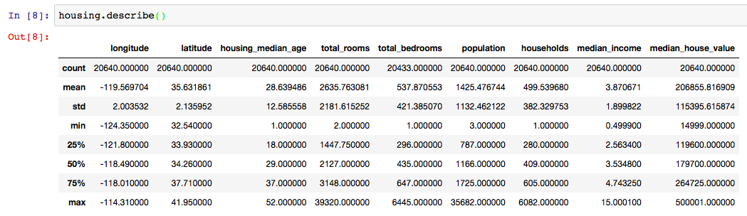
- There are 20,640 instances in the dataset
- the total_bed rooms attribute has only 20,433 non-null values, meaning that 207 districts are miss‐ ing this feature.
- All attributes are numerical, except the ocean_proximity field. Its type is object, so it could hold any kind of Python object, but since you loaded this data from a CSV file you know that it must be a text attribute.
The describe() method shows a summary of each numerical attributes
Another quick way to get a feel of the type of data you are dealing with is to plot a histogram for each numerical attribute.
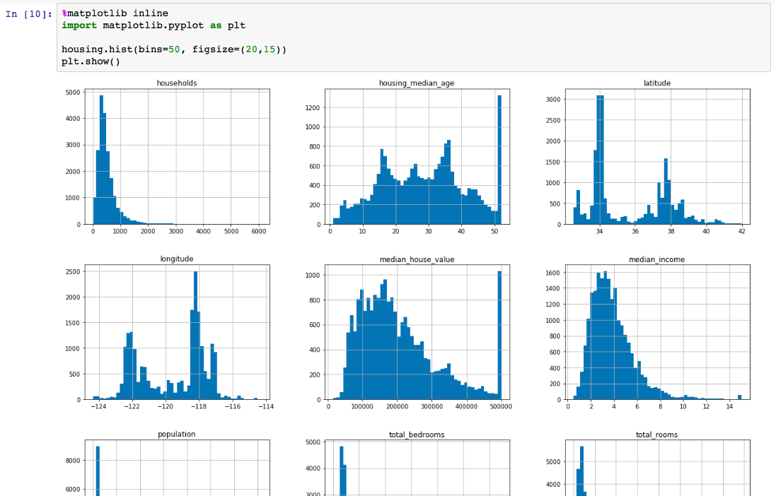
You need to specify which backend Matplotlib should use. The simplest option is to use Jupyter’s magic command %matplotlib inline. Plots are then rendered within the notebook itself.
Create a Test Set
Creating a test set is theoretically quite simple: just pick some instances randomly, typically 20% of the dataset
import numpy as np

def split_train_test(data, test_ratio):
    shuffled_indices = np.random.permutation(len(data))
    test_set_size = int(len(data) * test_ratio)
    test_indices = shuffled_indices[:test_set_size]
    train_indices = shuffled_indices[test_set_size:]
    return data.iloc[train_indices], data.iloc[test_indices]
- numpy.random.permutation() randomly permute a sequence, or return a permuted range.
- pandas.DataFrame.iloc() is purely integer-location based indexing for selection by position.
train_set, test_set = split_train_test(housing, 0.2)
print(len(train_set), "train +", len(test_set), "test")

16512 train + 4128 test
To ensure that the test set will remain consistent across multiple runs, even if you refresh the dataset, you could compute a hash of each instance’s identifier, keep only the last byte of the hash, and put the instance in the test set if this value is lower or equal to 51 (~20% of 256).
import hashlib

def test_set_check(identifier, test_ratio, hash):
    return hash(np.int64(identifier)).digest()[-1] < 256 * test_ratio

def split_train_test_by_id(data, test_ratio, id_column, hash=hashlib.md5):
    ids = data[id_column]
    in_test_set = ids.apply(lambda id_: test_set_check(id_, test_ratio, hash))
    return data.loc[~in_test_set], data.loc[in_test_set]
Python's hashlib module implements a common interface to many different secure hash and message digest algorithms.
- hashlib.md5() is the constructor for the hash algorithm MD5.
- digest() returns the digest of the strings passed to the update() method so far.
Python anonymous functions are defined using the lambda keyword.
- Syntax of Lambda Function in python
lambda arguments: expression
double = lambda x: x * 2
# Output: 10
print(double(5))

# Output: 10
lambda x: x * 2(5)
pandas.DataFrame.>apply(func, axis=0, broadcast=False, raw=False, reduce=None, args=(), **kwds)
- Applies function along input axis of DataFrame.
- Return type depends on whether passed function aggregates, or the reduce argument if the DataFrame is empty.
- With the usage of Lambda
          x  y
0  0.696469  1
1  0.286139  0
df['id'] = df['y'].apply(lambda d: "id_%d" % d)
          x  y    id
0  0.696469  1  id_1
1  0.286139  0  id_0
The housing dataset does not have an identifier column. The simplest solution is to use the row index as the ID:
housing_with_id = housing.reset_index() # adds an `index` column
train_set, test_set = split_train_test_by_id(housing_with_id, 0.2, "index")
- DataFrame.reset_index(level=None, drop=False, inplace=False, col_level=0, col_fill='')[source] When we reset the index, the old index is added as a column, and a new sequential index is used:
>>> df
         class  max_speed
falcon    bird      389.0
parrot    bird       24.0
lion    mammal       80.5
monkey  mammal        NaN

>>> df.reset_index()
    index   class  max_speed
0  falcon    bird      389.0
1  parrot    bird       24.0
2    lion  mammal       80.5
3  monkey  mammal        NaN
If this is not possible, then you can try to use the most stable features to build a unique identifier.
For example, a district’s latitude and longitude
housing_with_id["id"] = housing["longitude"] * 1000 + housing["latitude"]
train_set, test_set = split_train_test_by_id(housing_with_id, 0.2, "id")
Scikit-Learn provides a few functions to split datasets into multiple subsets in various ways. The simplest function is train_test_split() which is similar to split_train_test() defined earlier.
If your data set is large enough, you can consider the sample is uniformly distributed then sample it random;y.
If it is not, the data set is divided into homogeneous subgroups called strata, and the right number of instances is sampled from each stratum to guarantee that the test set is representative of the distribution .
You should not have too many strata, and each stratum should be large enough.
The following code creates an income category attribute by dividing the median income by 1.5 (to limit the number of income categories, the max. median_income is 15 in this case), and rounding up using ceil (to have discrete categories), and then merging all the categories greater than 5 into category 5:
housing["income_cat"] = np.ceil(housing["median_income"] / 1.5)
housing["income_cat"].where(housing["income_cat"] < 5, 5.0, inplace=True)
- numpy.ceil() Return the ceiling(天花板) of the input, element-wise. 傳回每個元素的最大整數.
>>> a = np.array([-1.7, -1.5, -0.2, 0.2, 1.5, 1.7, 2.0])
>>> np.ceil(a)
array([-1., -1., -0.,  1.,  2.,  2.,  2.])
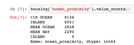
looking at the income category proportions in the full housing dataset:
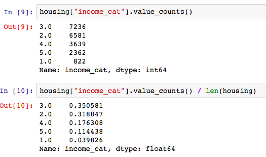
- Series.value_counts(normalize=False, sort=True, ascending=False, bins=None, dropna=True) Returns object containing counts of unique values. The resulting object will be in descending order so that the first element is the most frequently-occurring element. Excludes NA values by default.
Now, you can use Scikit-Learn’s StratifiedShuffleSplit class to provide train/test indices to split data in train/test sets.
This cross-validation object is a merge of StratifiedKFold and ShuffleSplit, which returns stratified randomized folds. The folds are made by preserving the percentage of samples for each class.
from sklearn.model_selection import StratifiedShuffleSplit

split = StratifiedShuffleSplit(n_splits=1, test_size=0.2, random_state=42) # create a split object
for train_index, test_index in split.split(housing, housing["income_cat"]):
        strat_train_set = housing.loc[train_index]
        strat_test_set = housing.loc[test_index]
- split(X, y, groups=None) Generate indices to split data into training and test set. X is the training data and y is the target variable for supervised learning problems.
>>> housing["income_cat"].value_counts() / len(housing)
3.0    0.350581
2.0    0.318847
4.0    0.176308
5.0    0.114438
1.0    0.039826
Name: income_cat, dtype: float64
To remove the income_cat attribute so the data is back to its original state:
for set in (strat_train_set, strat_test_set):
    set.drop(["income_cat"], axis=1, inplace=True)
- DataFrame.drop(labels=None, axis=0, index=None, columns=None, level=None, inplace=False, errors='raise') Return new object with labels(single label or list-like Index or column labels to drop.) in requested axis removed. Examples,
>>> df = pd.DataFrame(np.arange(12).reshape(3,4), columns=['A', 'B', 'C', 'D'])
>>> df
   A  B   C   D
0  0  1   2   3
1  4  5   6   7
2  8  9  10  11

#Drop columns

>>> df.drop(['B', 'C'], axis=1)
   A   D
0  0   3
1  4   7
2  8  11
>>> df.drop(columns=['B', 'C'])
   A   D
0  0   3
1  4   7
2  8  11

#Drop a row by index

>>> df.drop([0, 1])
   A  B   C   D
2  8  9  10  11
Discover and Visualize the Data to Gain Insights
Let’s create a copy so you can play with it without harming the training set:
housing = strat_train_set.copy()
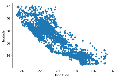
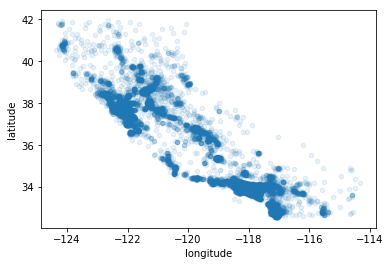
Visualizing Geographical Data
%matplotlib inline
housing.plot(kind="scatter", x="longitude", y="latitude")
Setting the alpha option to 0.1 makes it much easier to visualize the places where there is a high density of data points
%matplotlib inline
housing.plot(kind="scatter", x="longitude", y="latitude", alpha=0.1)
Looking for Correlations
We can compute the standard correlation coefficient (also called Pearson’s r) between every pair of attributes using the corr() method:
corr_matrix = housing.corr()
corr_matrix["median_house_value"].sort_values(ascending=False)
median_house_value 1.000000
median_income 0.687160
income_cat 0.642274
total_rooms 0.135097
housing_median_age 0.114110
households 0.064506
total_bedrooms 0.047689
population -0.026920
longitude -0.047432
latitude -0.142724
Name: median_house_value, dtype: float64
The correlation coefficient only measures linear correlations (“if x goes up, then y generally goes up/down”).
The correlation coefficient ranges from –1 to 1.
- the median house value tends to go up when the median income goes up
- prices have a slight tendency to go down when you go north(the "latitude")
Another way to check for correlation between attributes is to use Pandas’ scatter_matrix function, which plots every numerical attribute against every other numerical attribute.
We just focus on a few promising attributes that seem most correlated with the median housing value
from pandas.plotting import scatter_matrix

attributes = ["median_house_value", "median_income", "total_rooms", "housing_median_age"]
scatter_matrix(housing[attributes], figsize=(12, 8))
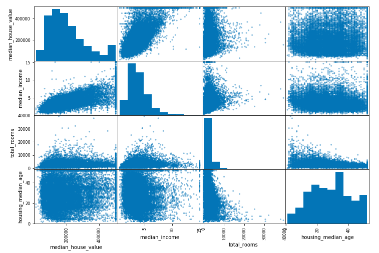
The main diagonal (top left to bottom right) would be full of straight lines if Pandas plotted each variable against itself.
Let’s zoom in on the correlation between "median_income"and "median_house_value"
housing.plot(kind="scatter", x="median_income", y="median_house_value", alpha=0.1)
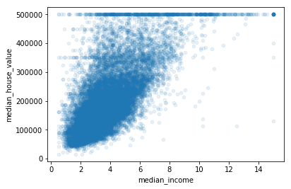
You may want to try removing the corresponding districts to prevent your algorithms from learning to reproduce these data quirks:
- a horizontal line at $500,000
- a horizontal line around $450,000
- a horizontal line around $350,000
Experimenting with Attribute Combinations
Some attributes are not directly correlated to the result so that you may try out various attribute combinations.
Let’s create these new attributes:
    housing["rooms_per_household"] = housing["total_rooms"]/housing["households"]
    housing["bedrooms_per_room"] = housing["total_bedrooms"]/housing["total_rooms"]
    housing["population_per_household"]=housing["population"]/housing["households"]
corr_matrix = housing.corr()
corr_matrix["median_house_value"].sort_values(ascending=False)

median_house_value          1.000000
median_income               0.687160
income_cat                  0.642274
rooms_per_household         0.146285
total_rooms                 0.135097
housing_median_age          0.114110
households                  0.064506
total_bedrooms              0.047689
population_per_household   -0.021985
population                 -0.026920
longitude                  -0.047432
latitude                   -0.142724
bedrooms_per_room          -0.259984
Name: median_house_value, dtype: float64
Prepare the Data for Machine Learning Algorithms
Let’s separate the predictors and the labels(answers)
housing = strat_train_set.drop("median_house_value", axis=1)
housing_labels = strat_train_set["median_house_value"].copy()
Data Cleaning
Most Machine Learning algorithms cannot work with missing features, so let’s create a few functions to take care of them.There are 3 ways to do that:
- Get rid of the corresponding districts housing.dropna(subset=["total_bedrooms"])
- Get rid of the whole attribute housing.drop("total_bedrooms", axis=1)
- Set the values to some value (zero, the mean, the median, etc.). median = housing["total_bedrooms"].median() housing["total_bedrooms"].fillna(median)
Scikit-Learn provides a handy class to take care of missing values: Imputer.
from sklearn.preprocessing import Imputer

imputer = Imputer(strategy="median")
housing_num = housing.drop("ocean_proximity", axis=1)
Now you can fit the imputer instance to the training data
imputer.fit(housing_num)
imputer.statistics_

array([ -118.51  ,    34.26  ,    29.    ,  2119.5   ,   433.    ,
        1164.    ,   408.    ,     3.5409,     3.    ])
Now you can transform the training set by replacing missing values by the learned medians:
X = imputer.transform(housing_num)
To create a DataFrame/Series, you must convert the Imputer output to a list and use the resulting list as input to DataFrame()/Series().
housing_tr = pd.DataFrame(X, columns=housing_num.columns)
The main design principles in Scikit-Learn are:
- Consistency All objects within scikit-learn share a consistent and simple interfaces:
- Estimators In machine learning, a hyperparameter is a parameter whose value is set before the learning process begins. By contrast, the values of other parameters are derived via training. Any object that can estimate some parameters based on a dataset is called an estimator (e.g., an imputer is an estimator). The actual learning in the estimation is performed by the fit() method which learns a model from the data training set, and it takes only a dataset as a parameter (or two for supervised learning algorithms; the second dataset contains the labels). Any other parameter needed to guide the estimation process is considered a hyperparameter (such as an imputer’s strategy), and it must be set as an instance variable (generally via a constructor parameter).
- Transformers Since it is common to modify or filter data before feeding it to a learning algorithm, some estimators in the library implement a transformer interface which defines a transform method. Preprocessing, feature selection, feature extraction and dimensionality reduction algorithms are all provided as transformers within the library. The transformation is performed by the transform() method with the dataset to transform as a parameter. It returns the transformed dataset. This transformation generally relies on the learned parameters, as is the case for an imputer. All transformers also have a convenience method called fit_transform() that is equivalent to calling fit() and then transform() (but sometimes fit_transform() is optimized and runs much faster).
- Predictors Some estimators are capable of making predictions given a dataset; they are called predictors.A predictor has a predict() method that takes a dataset of new instances and returns a dataset of corresponding predictions. It also has a score() method that measures the quality of the predictions given a test set (and the corresponding labels in the case of supervised learning algorithms).
from sklearn.pseudoModule import pseudoModel

pseudoObject = pseudoModelConstructor()
pseudoObject.fit(X_train, y_train)
X_train = pseudoObject.transform(X train)
X_test = pseudoObject.transform(X test)
y_pred = pseudoObject.predict(X_test)
Handling Text and Categorical Attributes
We can convert text labels to numbers because most Machine Learning algorithms prefer to work with numbers.
Scikit-Learn provides a transformer for this task called LabelEncoder:
from sklearn.preprocessing import LabelEncoder

encoder = LabelEncoder()
housing_cat = housing["ocean_proximity"]
housing_cat_encoded = encoder.fit_transform(housing_cat)
housing_cat_encoded

array([0, 0, 4, ..., 1, 0, 3])
print(encoder.classes_)

['<1h bay="" code="" ocean="">ML algorithms will assume that two nearby values are more similar than two distant values.(Obviously this is not the case)
To fix this issue, one-hot encoding is used. Scikit-Learn provides a OneHotEncoder encoder to convert integer categorical values into one-hot vectors.
Note that fit_transform() expects a 2D array, but housing_cat_encoded is a 1D array, so we need to reshape it:
from sklearn.preprocessing import OneHotEncoder

encoder = OneHotEncoder()
housing_cat_1hot = encoder.fit_transform(housing_cat_encoded.reshape(-1,1))

housing_cat_1hot
<16513x5 sparse matrix of type ''
             with 16513 stored elements in Compressed Sparse Row format>
If you really want to con‐ vert it to a (dense) NumPy array, just call the toarray() method:
housing_cat_1hot.toarray()

array([[ 0., 1., 0., 0., 0.],
       [ 0., 1., 0., 0., 0.],
       [ 0., 0., 0., 0., 1.],
       ...,
       [ 0.,  1.,  0.,  0.,  0.],
       [ 1.,  0.,  0.,  0.,  0.],
       [ 0.,  0.,  0.,  1.,  0.]])
from sklearn.preprocessing import LabelBinarizer

encoder = LabelBinarizer()
housing_cat_1hot = encoder.fit_transform(housing_cat)
Custom Transformers
You will want your transformer to work seamlessly with Scikit-Learn func‐ tionalities (such as pipelines), all you need is to create a class and implement three methods: fit() (returning self), transform(), and fit_transform().Feature Scaling
Transformation Pipelines
Scikit-Learn provides the Pipeline class to help with many data transformation steps that need to be executed in the right order. The Pipeline constructor takes a list of name/estimator pairs defining a sequence of steps.
from sklearn.pipeline import Pipeline
from sklearn.preprocessing import StandardScaler

num_pipeline = Pipeline([
            ('imputer', Imputer(strategy="median")),
            ('attribs_adder', CombinedAttributesAdder()),
            ('std_scaler', StandardScaler()),
        ])
housing_num_tr = num_pipeline.fit_transform(housing_num)
All but the last estimator must be transformers.
When you call the pipeline’s fit() method, it calls fit_transform() sequentially on all transformers, passing the output of each call as the parameter to the next call, until it reaches the final estimator, for which it just calls the fit() method.

留言
George Ng
Thanks for comment.
This is my notebook about the reading of the book "Hands-On Machine Learning with Scikit-Learn and TensorFlow".
We are standing on the shoulders of giants.
My current work is not related to machine learning.
I am still learning related knowledge when I have free time.
Regards
Jerry
Thanks For Sharing
Machine learning in Vijayawada