Deep Learning with Python
The code examples use the Python deep-learning framework Keras, with Tensor- Flow as a backend engine. Keras, one of the most popular and fastest-growing deep- learning frameworks, is widely recommended as the best tool to get started with deep learning.
PART 1 Fundamental of Deep Learning
1 What is deep learning?
1.1 Artificial intelligence, machine learning, and deep learning
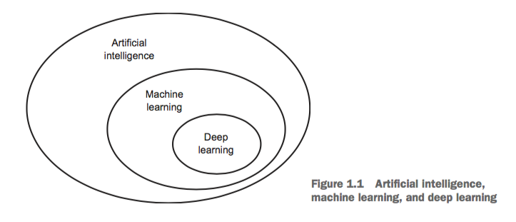
1.1.2 Machine learning
With machine learning, humans input data as well as the answers expected from the data, and out come the rules. These rules can then be applied to new data to produce original answers.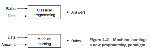
A machine-learning system is trained rather than explicitly programmed.
1.1.3 Learning representations from data
To do machine learning, we need three things:- Input data
- Examples of the expected output for the input data
- A way to measure whether the algorithm is doing a good job The measurement is used as a feedback signal to adjust the way the algorithm works. This adjustment step is what we call learning.
1.1.4 The “deep” in deep learning
The deep in deep learning stands for this idea of successive layers of representations. How many layers contribute to a model of the data is called the depth of the model.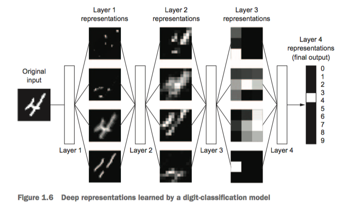
1.1.5 Understanding how deep learning works, in three figures
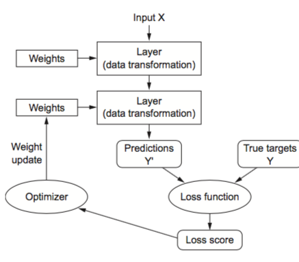
The machine learning is about mapping inputs (such as images) to targets (such as the label “cat”), this input-to-target mapping via a deep sequence of simple data transformations (layers) and that these data transformations are learned by exposure to examples.
What a layer to do about its input data is stored in the layer’s weights, the transformation implemented by a layer is parameterized by its weights.
In this context, learning means finding a set of values for the weights of all layers in a network, such that the network will correctly map example inputs to their associated targets.
The loss function(objective function) is to measure how far (score) this output is from what you expected.
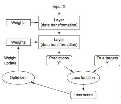
The fundamental trick in deep learning is to use this score as a feedback signal to adjust the value of the weights a little, in a direction that will lower the loss score for the current sample. This adjustment is the job of the optimizer, which implements what’s called the Backpropagation algorithm: the central algorithm in deep learning.
Initially, the weights of the network are assigned random values, with every sample the network processes, the weights are adjusted a little in the correct direction, and the loss score decreases. This is the training loop, repeated a sufficient number of times, yields weight values that minimize the loss function.
1.2 Before deep learning: a brief history of machine learning
Most of the machine-learning algorithms used in the industry today aren’t deep-learning algorithms, deep learning isn’t always the right tool for the job — sometimes there isn’t enough data for deep learning to be applicable, and sometimes the problem is better solved by a different algorithm.1.2.1 Probabilistic modeling
1.2.2 Early neural networks
1.2.3 Kernel methods
Kernel methods are a group of classification algorithms, the best known of which is the support vector machine (SVM).SVMs aim at solving classification problems by finding good decision boundaries between two sets of points belonging to two different categories.
Decision trees, random forests, and gradient boosting machines
Decision trees are flowchart-like structures that let you classify input data points or pre- dict output values given inputs1.2.5 Back to neural networks
Since 2012, deep convolutional neural networks (convnets) have become the go-to algorithm for all computer vision tasks1.2.6 What makes deep learning different
The primary reason deep learning took off so quickly is that it offered better performance on many problems.1.2.7 The modern machine-learning landscape
A great way to get a sense of the current landscape of machine-learning algorithms and tools is to look at machine-learning competitions on Kaggle. Kaggle is a platform for predictive modelling and analytics competitions in which statisticians and data miners compete to produce the best models for predicting and describing the datasets uploaded by companies and users.1.3 Why deep learning? Why now?
The two key ideas of deep learning for computer vision — convolutional neural networks and backpropagation — were already well understood in 1989. So why did deep learning only take off after 2012?
The real bottlenecks throughout the 1990s and 2000s were data and hardware.
1.3.1 Hardware
- NVIDIA launched CUDA (https://developer.nvidia.com/about-cuda), a programming interface for its line of GPUs.
- Google revealed its tensor processing unit (TPU) project: a new chip design developed from the ground up to run deep neural networks, which is reportedly 10 times faster and far more energy efficient than top-of-the-line GPUs.
1.3.2 Data
If deep learning is the steam engine of this revolution, then data is its coal: the raw material that powers our intelligent machines, without which nothing would be possible.If there’s one dataset that has been a catalyst for the rise of deep learning, it’s the ImageNet dataset, consisting of 1.4 million images that have been hand annotated with 1,000 image categories (1 category per image).
1.3.3 Algorithms
The key issue was that of gradient propagation through deep stacks of layers. The feedback signal used to train neural networks would fade away as the number of layers increased.2 Before we begin: the mathematical building blocks of neural networks
2.1 A first look at a neural network
In machine learning, a category in a classification problem is called a class. Data points are called samples. The class associated with a specific sample is called a label.
The problem we’re trying to solve here is to classify grayscale images of handwritten digits (28 × 28 pixels) into their 10 categories (0 through 9). We’ll use the MNIST dataset assembled by the National Institute of Standards and Technology (the NIST in MNIST):
- a set of 60,000 training images
- a set of 10,000 test images
- train_images and train_labels form the training set
>>> train_images.shape
(60000, 28, 28)
>>> len(train_labels)
60000
>>> train_labels
array([5, 0, 4, ..., 5, 6, 8], dtype=uint8)
>>> test_images.shape
(10000, 28, 28)
>>> len(test_labels)
10000
>>> test_labels
array([7, 2, 1, ..., 4, 5, 6], dtype=uint8)
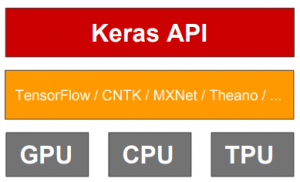
Keras is a high-level neural networks API, written in Python and capable of running on top of TensorFlow, CNTK, or Theano.
To set up Keras
   pip install keras
   pip install tensorflow
   pip list | grep -i keras
   pip list | grep -i tensorflow
>>> import tensorflow as tf
Illegal instruction (core dumped)
Breaking Changes
Prebuilt binaries are now built against CUDA 9.0 and cuDNN 7.
Prebuilt binaries will use AVX instructions. This may break TF on older CPUs.
You have at least two options:
- Use tensorflow 1.5 or older You will miss out on new features, but most basic features and documentations are not that different.
- Build from source
Try to uninstall them then downgrade to a working version 1.5:
  sudo pip3 uninstall Tensorflow
  sudo pip install tensorflow==1.5
   conda install -c anaconda tensorflow
   conda install -c anaconda keras
   conda install -c anaconda opencv # 3.4.2
#   conda install -c conda-forge opencv=3.2.0 # 4.1.1
   pip install opencv-python
   pip install opencv-contrib-python
Here is an example of the flow:
- Loading the MNIST dataset in Keras MNIST database of handwritten digits is a dataset of 60,000 28x28 grayscale images of the 10 digits, along with a test set of 10,000 images.
- train_images, test_images: uint8 array of grayscale image data with shape (num_samples, 28, 28).
- train_labels, test_labels: uint8 array of digit labels (integers in range 0-9) with shape (num_samples,).
- Build the network architecture This network consists of a sequence of 2 Dense layers, which are densely connected (also called fully connected) neural layers.
- Pass an input_shape argument to the first layer.
- Some 2D layers, such as Dense, support the specification of their input shape via the argument input_dim
- If you ever need to specify a fixed batch size for your inputs (this is useful for stateful recurrent networks), you can pass a batch_size argument to a layer. If you pass both batch_size=32 and input_shape=(6, 8) to a layer, it will then expect every batch of inputs to have the batch shape (32, 6, 8).
- units is a positive integer which decides the dimensionality of the output space.
- activation is the element-wise activation function passed as the activation argument
- kernel is a weights matrix created by the layer
- bias is a bias vector created by the layer (only applicable if use_bias is True).
- The compilation step Before training a model, you need to configure the learning process, which is done via the compile method.
- An optimizer The mechanism through which the network will update itself based on the data it sees and its loss function. This could be the string identifier of an existing optimizer (such as rmsprop oradagrad), or an instance of the Optimizer class. See: optimizers.
- A loss function How the network will be able to measure its performance on the training data, and thus how it will be able to steer itself in the right direction. This is the objective that the model will try to minimize. It can be the string identifier of an existing loss function (such as categorical_crossentropy or mse), or it can be an objective function.
- A list of metrics Metrics to monitor during training and testing. For any classification problem you will want to set this to metrics=['accuracy']. A metric could be the string identifier of an existing metric or a custom metric function.
- Preparing the image data We transform it into a float32 array of shape (60000, 28 * 28) with values between 0 and 1.
- Preparing the labels
- y is a class vector(integers from 0 to num_classes) to be converted .
- num_classes total number of classes.
- dtype The data type expected by the input, as a string (float32, float64, int32...)
# 1 Loading the MNIST dataset in Keras
from keras.datasets import mnist
(train_images, train_labels), (test_images, test_labels) = mnist.load_data()
# 2 Build the network architecture
from keras import models
from keras import layers
network = models.Sequential()
network.add(layers.Dense(512, activation='relu', input_shape=(28 * 28,)))
network.add(layers.Dense(10, activation='softmax'))
output = activation( dot(input, kernel) + bias )
keras.layers.Dense(units, activation=None, use_bias=True, kernel_initializer='glorot_uniform', bias_initializer='zeros', kernel_regularizer=None, bias_regularizer=None, activity_regularizer=None, kernel_constraint=None, bias_constraint=None)
# 3 The compilation step
network.compile(optimizer='rmsprop',
                loss='categorical_crossentropy',
                metrics=['accuracy'])
#4 Preparing the image data
train_images = train_images.reshape((60000, 28 * 28))
train_images = train_images.astype('float32') / 255
test_images = test_images.reshape((10000, 28 * 28))
test_images = test_images.astype('float32') / 255
>>>
>>> x = np.array([1, 2, 2.5])
>>> x
array([1. ,  2. ,  2.5])
>>>
>>> x.astype(int)
array([1, 2, 2])
#5 Preparing the labels
from keras.utils import to_categorical

train_labels = to_categorical(train_labels)
test_labels = to_categorical(test_labels)
> labels
array([0, 2, 1, 2, 0])
# `to_categorical` converts this into a matrix with as many
# columns as there are classes. The number of rows
# stays the same.
> to_categorical(labels)
array([[ 1.,  0.,  0.],
       [ 0.,  0.,  1.],
       [ 0.,  1.,  0.],
       [ 0.,  0.,  1.],
       [ 1.,  0.,  0.]], dtype=float32)
使用summary指令review一下整個model:
network.summary()
Layer (type)                 Output Shape              Param #
=================================================================
dense_1 (Dense)              (None, 512)               401920
_________________________________________________________________
dense_2 (Dense)              (None, 10)                5130
=================================================================
Total params: 407,050
Trainable params: 407,050
Non-trainable params: 0
- 401920 (28 x 28 + 1 ) x 512 = 401920
- 5130 (512 + 1 ) x 10 = 5130
Keras models are trained on Numpy arrays of input data and labels.
We’re now ready to train the network by calling the network’s fit method in Keras:
fit(self, x=None, y=None, batch_size=None, epochs=1, verbose=1, callbacks=None, validation_split=0.0, validation_data=None, shuffle=True, class_weight=None, sample_weight=None, initial_epoch=0, steps_per_epoch=None, validation_steps=None)
- x Numpy array of training data.
- y Numpy array of target (label) data.
- batch_size Integer or None. Number of samples per gradient update. If unspecified, it will default to 32.
- epochs Integer. Number of epochs to train the model. An epoch is an iteration over the entire input and target data provided. Note that in conjunction with initial_epoch, epochs is to be understood as "final epoch". The model is not trained for a number of iterations given by epochs, but merely until the epoch of index epochs is reached.
- shuffle Boolean (whether to shuffle the training data before each epoch) or str (for 'batch'). 'batch' is a special option for dealing with the limitations of HDF5 data; it shuffles in batch-sized chunks
fit() returns a History object.
Its History.history attribute is a record of training loss values and metrics values at successive epochs, as well as validation loss values and validation metrics values (if applicable).
>>> train_history = network.fit(train_images, train_labels, epochs=5, batch_size=128)

Epoch 1/5
60000/60000 [==============================] - 7s 118us/step - loss: 0.2550 - acc: 0.9260
Epoch 2/5
60000/60000 [==============================] - 7s 109us/step - loss: 0.1028 - acc: 0.9697
Epoch 3/5
60000/60000 [==============================] - 7s 110us/step - loss: 0.0682 - acc: 0.9797
Epoch 4/5
60000/60000 [==============================] - 7s 111us/step - loss: 0.0501 - acc: 0.9851
Epoch 5/5
60000/60000 [==============================] - 7s 115us/step - loss: 0.0377 - acc: 0.9886
We quickly reach an accuracy of 0.9886 (98.9%) on the training data.
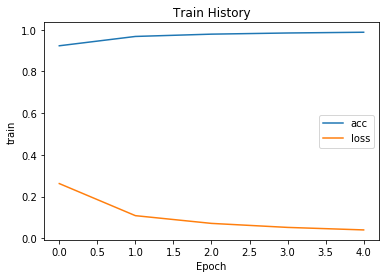
每訓練完一個週期,會計算此週期的accuracy與loss放到train_history.history這個dictionary object中。
{'acc': [0.99143333333333339,
  0.99368333336512249,
  0.99528333330154417,
  0.99626666663487751,
  0.99703333333333333],
 'loss': [0.029321372731526692,
  0.022051296432067949,
  0.016661394806827108,
  0.01325423946591715,
  0.010353616964444519]}
import matplotlib.pyplot as plt

def show_train_history(train_history, label_1, label_2):
    plt.plot(train_history.history[label_1])
    plt.plot(train_history.history[label_2])
    plt.title('Train History')
    plt.ylabel('train')
    plt.xlabel('Epoch')
    plt.legend([label_1, label_2], loc='center right')
    plt.show()
show_train_history(train_history, 'acc','loss')
現在,利用訓練好的模型來預測test dataset:
    predicted_results = network.predict(test_images, verbose=1)

predicted_results[0]
array([  3.35639416e-12,   4.17718540e-13,   9.10662337e-08,
         1.63431287e-05,   1.50763562e-18,   1.97378971e-11,
         1.31892617e-19,   9.99983549e-01,   4.16868137e-11,
         2.15591989e-08], dtype=float32)

test_labels[0]
array([ 0.,  0.,  0.,  0.,  0.,  0.,  0.,  1.,  0.,  0.])
最後,我們使用test dataset來評估模型的準確率:
evaluate(self, x=None, y=None, batch_size=None, verbose=1, sample_weight=None, steps=None)
- x input data, as a Numpy array or list of Numpy arrays (if the model has multiple inputs).
- y labels, as a Numpy array.
- batch_size Integer. If unspecified, it will default to 32.
>>> test_loss, test_acc = network.evaluate(test_images, test_labels)
>>> print('test_acc:', test_acc)

test_acc: 0.981
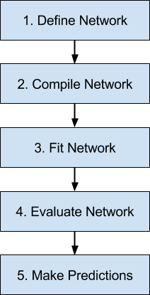
The 5 steps in the neural network model life-cycle in Keras:
2.2 Data representations for neural networks
In mathematics, tensors are geometric objects that describe linear relations between geometric vectors, scalars, and other tensors.In general, all current machine-learning systems use tensors as their basic data structure. A tensor is a container for data.
2.2.1 Scalars (0D tensors)
A tensor that contains only one number is called a scalar (or scalar tensor, or 0-dimensional tensor, or 0D tensor).The number of axes of a tensor is also called its rank.
2.2.2 Vectors (1D tensors)
An array of numbers is called a vector, or 1D tensor. A 1D tensor is said to have exactly one axis.2.2.3 Matrices (2D tensors)
An array of vectors is a matrix, or 2D tensor. A matrix has two axes (often referred to rows and columns).2.2.4 3D tensors and higher-dimensional tensors
If you pack such matrices in a new array, you obtain a 3D tensor. In deep learning, you’ll generally manipulate tensors that are 0D to 4D, although you may go up to 5D if you process video data.2.2.5 Key attributes
A tensor is defined by three key attributes:- Number of axes (rank) This is also called the tensor’s ndim in Python libraries such as Numpy.
- Shape This is a tuple of integers that describes how many dimensions the tensor has along each axis. A vector has a shape with a single element, such as (5,), whereas a scalar has an empty shape, ().
- Data type (usually called dtype in Python libraries)
 print(train_images.ndim)
 3
 print(train_images.shape)
 (60000, 28, 28)
 print(train_images.ndim)
 2
 print(train_images.shape)
 (60000, 784)
2.2.6 Manipulating tensors in Numpy
Selecting specific elements in a tensor is called tensor slicing.- Select image digits #10 to #100
>>> my_slice = train_images[10:100]
>>> print(my_slice.shape)
(90, 28, 28)
my_slice = train_images[:, 14:, 14:]
my_slice = train_images[:, 7:-7, 7:-7]
2.2.7 The notion of data batches
In general, the first axis (axis 0, because indexing starts at 0) in all data tensors you’ll come across in deep learning will be the samples axis.The deep-learning models don’t process an entire dataset at once; rather, they break the data into small batches. When considering such a batch tensor, the first axis (axis 0) is called the batch axis or batch dimension.
For the batch size of 128, the n-th batch samples in the MNIST dataset:
batch = train_images[128 * n:128 * (n + 1)]
2.2.8 Real-world examples of data tensors
The data you’ll manipulate will almost always fall into one of the following categories:- Vector data 2D tensors of shape (samples, features)
- Timeseries data or sequence data 3D tensors of shape (samples, timestamps, features)
- Images 4D tensors of shape(samples,height,width,channels) or (samples, channels, height, width)
- Video 5D tensors of shape (samples, frames, height, width, channels) or (samples, frames, channels, height, width)
2.2.9 Vector data
Examples:- Each person can be characterized as a vector of 3 feature values: age, ZIP code, and income An entire dataset of 100,000 people can be stored in a 2D tensor of shape (100000, 3).
- Each document can be characterize by the counts of how many times each word appears in it (out of a dictionary of 20,000 common words). An entire dataset of 500 documents can be stored in a tensor of shape (500, 20000).
| person#1 | age_1 | ZIP_1 | income_1 |
| person#2 | age_2 | ZIP_2 | income_2 |
| . | . | . | . |
| person#100000 | age_100000 | ZIP_100000 | income_100000 |
2.2.10 Timeseries data or sequence data
Whenever time matters in your data , it makes sense to store it in a 3D tensor with an explicit time axis. The time axis is always the second axis (axis of index 1), by convention.Examples:
- A day's stock price is recorded every minute: highest, lowest and the current price. An entire dataset of 6.5 hours trading time(390 minutes) for 250 days can be stored in a 3D tensor of shape(250, 390, 3).
2.2.11 Image data
Images typically have three dimensions: height, width, and color depth.- A batch of 128 grayscale images of size 256 × 256 could thus be stored in a tensor of shape (128, 256, 256, 1)
- a batch of 128 color images could be stored in a tensor of shape (128, 256, 256, 3)
2.2.12 Video data
Because each frame can be stored in a 3D tensor (height, width, color_depth), a sequence of frames can be stored in a 4D tensor (frames, height, width, color_depth), and thus a batch of different videos can be stored in a 5D tensor of shape (samples, frames, height, width, color_depth).2.3 The gears of neural networks: tensor operations
Element-wise operations
Element-wise operations are operations that are applied independently to each entry in the tensors.If you want to write a naive Python implementation of an element-wise operation, you use a for loop.
As ReLU (Rectified Linear Unit) function as an example: 輸入超過0, 輸出結果就是輸入; 輸入小於0就輸出0.
The naive Python implementation of an element-wise ReLu operation:
def naive_relu(x):
    assert len(x.shape) # x is a 2D Numpy tensor.
    x = x.copy() # Avoid overwriting the input
    for i in range(x.shape[0]):
        for j in range(x.shape[1]):
            x[i, j] = max(x[i, j], 0)
    return x
In practice, when dealing with Numpy arrays, these operations are available as well optimized built-in Numpy functions. So, in Numpy, you can do the following element-wise operation,
import numpy as np

z = x + y             #  Element-wise addition
z = np.maximum(z, 0.) #  Element-wise function
2.3.2 Broadcasting
What happens with element-wise operations when the shapes of the two tensors are different?When possible, and if there’s no ambiguity, the smaller tensor will be broadcasted to match the shape of the larger tensor. Broadcasting consists of two steps:
- Axes (called broadcast axes) are added to the smaller tensor to match the ndim of the larger tensor.
- The smaller tensor is repeated alongside these new axes to match the full shape of the larger tensor.
2.3.3 Tensor dot
In mathematics, the dot product or scalar product is an algebraic operation that takes two equal-length sequences of numbers (usually coordinate vectors) and returns a single number. In Euclidean geometry, the dot product of the Cartesian coordinates of two vectors is widely used and often called inner product (or rarely projection product)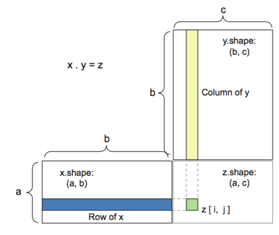
You can take the dot product of two matrices x and y (dot(x, y)) if and only if x.shape[1] == y.shape[0]. The result is a matrix with shape (x.shape[0], y.shape[1]), where the coefficients are the vector products between the rows of x and the columns of y.
2.3.4 Tensor reshaping
Reshaping a tensor means rearranging its rows and columns to match a target shape.2.3.6 A geometric interpretation of deep learning
Neural networks consist entirely of chains of tensor operations and that all of these tensor operations are just geometric transformations of the input data.2.4 The engine of neural networks: gradient-based optimization
Each neural layer transforms its input data.
The transformation is depended on the weights or trainable parameters of the layer.
These weights contain the information learned by the network from exposure to training data.
Initially, these weight matrices are filled with small random values (a step called random initialization).
What comes next is to gradually adjust these weights, based on a feedback signal. This gradual adjustment, also called training, is basically the learning that machine learning is all about.
This happens within what’s called a training loop, these steps are repeated as long as necessary:
- Draw a batch of training samples x and corresponding targets y.
- Run the network on x (a step called the forward pass) to obtain predictions y_pred.
- Compute the loss of the network on the batch, a measure of the mismatch between y_pred and y.
- Update all weights of the network in a way that slightly reduces the loss on this batch.
A much better approach is to take advantage of the fact that all operations used in the network are differentiable, and compute the gradient of the loss with regard to the network’s coefficients. You can then move the coefficients in the opposite direction from the gradient, thus decreasing the loss.
2.4.1 What’s a derivative?
If you want to reduce the value of f(x), you just need to move x a little in the opposite direction from the derivative.2.4.2 Derivative of a tensor operation: the gradient
With a function f(W) of a tensor, you can reduce f(W) by moving W in the opposite direction from the gradient: for example,
W1 = W0 - step * gradient(f)(W0)
where step is a small scaling factor.
2.4.3 Stochastic gradient descent
If you update the weights in the opposite direction from the gradient, the loss will be a little less every time.
This is called mini-batch stochastic gradient descent (mini- batch SGD). The term stochastic refers to the fact that each batch of data is drawn at random (stochastic is a scientific synonym of random).
If the parameter under consideration were being optimized via SGD with a small learning rate, then the optimization process would get stuck at the local minimum instead of making its way to the global minimum.
You can avoid such issues by using momentum.
Momentum is implemented by moving the ball at each step based not only on the current slope value (current acceleration)
but also on the current velocity (resulting from past acceleration).
past_velocity = 0
momentum = 0.1 # Constant momentum factor

while loss > 0.01:  # Optimization loop
    w, loss, gradient = get_current_parameters()
    velocity = past_velocity * momentum + learning_rate * gradient
    w = w + momentum * velocity - learning_rate * gradient
    past_velocity = velocity
    update_parameter(w)
2.4.4 Chaining derivatives: the Backpropagation algorithm
Chain rule:
f'(x) = f'(g) * g'(x)
f(W1, W2, W3) = a( W1, b( W2, c(W3) ) )
Thanks to symbolic differentiation, you’ll never have to implement the Backpropagation algorithm by hand.
2.5 Looking back at our first example
3 Getting started with neural networks
This chapter covers the three most common use cases of neural networks:
- binary classification Classifying results as positive or negative.
- multiclass classification
- scalar regression Estimating the number of a target.
3.1 Anatomy of a neural network
Training a neural network revolves around the following objects:
- Layers, which are combined into a network (or model)
- The input data and corresponding targets
- The loss function, which defines the feedback signal used for learning
- The optimizer, which determines how learning proceeds
3.1.1 Layers: the building blocks of deep learning
Every layer will only accept input tensors of a certain shape and will return output tensors of a certain shape.
For ex.,
from keras import layers

layer = layers.Dense(32, input_shape=(784,))
- The created layer will only accept as input 2D tensors where the first dimension(axis 0) is 784( 28 x 28 ).
- This layer will return a tensor where the first dimension has been transformed to be 32.
- This layer can only be connected to a downstream layer that expects 32 dimensional vectors as its input.
from keras import models
from keras import layers
model = models.Sequential()
model.add(layers.Dense(32, input_shape=(784,)))
model.add(layers.Dense(32))
3.1.2 Models: networks of layers
Picking the right network architecture is more an art than a science, only practice can help you become a proper neural-network architect.
3.1.3 Loss functions and optimizers: keys to configuring the learning process
Once the network architecture is defined, you still have to choose two more things:
- Loss function (objective function) The quantity that will be minimized during training. It represents a measure of success for the task at hand.
- Optimizer Determines how the network will be updated based on the loss function. It implements a specific variant of stochastic gradient descent ( SGD ).
3.2 Introduction to Keras
Keras(https://keras.io) is a deep-learning framework for Python that provides a convenient way to define and train almost any kind of deep-learning model.
3.2.1 Keras, TensorFlow, Theano, and CNTK
Keras is a model-level library, providing high-level building blocks for developing deep-learning models.
Keras relies on a specialized, well-optimized tensor library to do so, serving as the backend engine of Keras.
Several different backend engines(TensorFlow, Microsoft Cognitive Toolkit/CNTK , Caffe, Theano, Torch, Pytotch) can be plugged seamlessly into Keras.
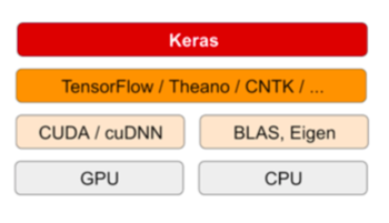
Any piece of code that you write with Keras can be run with any of these backends without having to change anything in the code.
Keras is able to run seamlessly on both CPUs and GPUs.
- running on CPU TensorFlow is itself wrapping a low-level library for tensor operations called Eigen (http://eigen.tuxfamily.org).
- running on GPU TensorFlow wraps a library of well-optimized deep-learning operations called the NVIDIA CUDA Deep Neural Network library (cuDNN ).
3.2.2 Developing with Keras: a quick overview
The typical Keras workflow looks just like:
- Define your training data: input tensors and target tensors.
- Define a network of layers (or model ) that maps your inputs to your targets. There are two ways to define a model: using the Sequential class (only for linear stacks of layers, which is the most common network architecture by far) or the functional API.
- Configure the learning process by choosing a loss function, an optimizer, and some metrics to monitor. The learning process is configured in the compilation step. For ex.,
- Iterate on your training data by calling the fit() method of your model. Finally, the learning process consists of passing Numpy arrays of input data (and the corresponding target data) to the model via the fit() method
| Sequential class | functional API |
|---|---|
from keras import models from keras import layers model = models.Sequential() model.add(layers.Dense(32, activation='relu', input_shape=(784,))) model.add(layers.Dense(10, activation='softmax')) | from keras import models from keras import layers input_tensor = layers.Input(shape=(784,)) x = layers.Dense(32, activation='relu')(input_tensor) output_tensor = layers.Dense(10, activation='softmax')(x) model = models.Model(inputs=input_tensor, outputs=output_tensor) |
from keras import optimizers

model.compile(optimizer=optimizers.RMSprop(lr=0.001),
              loss='mse',
              metrics=['accuracy'])
model.fit(input_tensor, target_tensor, batch_size=128, epochs=10)3.3 Setting up a deep-learning workstation
It’s highly recommended that you run deep-learning code on a modern neural network processor because some applications will be excruciatingly slow on CPU , even a fast multicore CPU .
Running cloud GPU instances ( AWS EC2 GPU instance or on Google Cloud Platform) can become expensive over time.
3.3.1 Jupyter notebooks: the preferred way to run deep-learning experiments
It allows you to break up long experiments into smaller pieces that can be executed independently, which makes development interactive and means you don’t have to rerun all of your previous code if something goes wrong late in an experiment.
3.3.2 Getting Keras running: two options
- Use the official EC2 Deep Learning AMI(https://aws.amazon.com/amazon-ai/amis) and run Keras experiments as Jupyter notebooks on EC2 .
- Install everything from scratch on a local Unix workstation. Do this if you already have a high-end NVIDIA GPU .
3.3.3 Running deep-learning jobs in the cloud: pros and cons
3.3.4 What is the best GPU for deep learning?
Using a GPU isn’t strictly necessary, but it’s strongly recommended.
You may sometimes have to wait for several hours for a model to train, instead of mere minutes on a good GPU .
nVidia's GPU
Modern deep-learning frameworks can only run on NVIDIA cards.To use your NVIDIA GPU for deep learning, you need to install two things:- CUDA A set of drivers for your GPU that allows it to run a low-level programming language for parallel computing.
- cu DNN A library of highly optimized primitives for deep learning. When using cu DNN and running on a GPU , you can typically increase the training speed of your models by 50% to 100%.
Please consult the TensorFlow website for detailed instructions about which versions are currently recommended.
Intel's TPU
Coral is a new platform, but it’s designed to work seamlessly with TensorFlow.To bring TensorFlow models to Coral you can use TensorFlow Lite, a toolkit for running machine learning inference on edge devices.
- Pre-trained models The Coral website provides pre-trained TensorFlow Lite models that have been optimized to use with Coral hardware.
- Retrain a model You can customize Coral’s pre-trained machine learning models to recognize your own images and objects. To do this, follow the instructions in Retrain an existing model.
- Build your own TensorFlow model You can follow the steps in Build a new model for the Edge TPU. Note that your model must meet the Model requirements. To prepare your model for the Edge TPU,
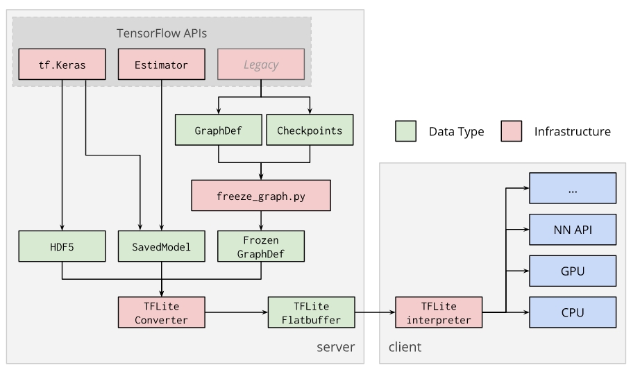
- You’ll first convert and optimize it for edge devices with the TensorFlow Lite Converter.
The TensorFlow Lite converter is used to convert TensorFlow models into an optimized FlatBuffer format, so that they can be used by the TensorFlow Lite interpreter.
The converter supports the following input formats:
- SavedModels
- Frozen GraphDef: Models generated by freeze_graph.py.
- tf.keras HDF5 models.
- Any model taken from a tf.Session (Python API only).
The TensorFlow Lite Converter can perform quantization on any trained TensorFlow model. You can read more about this technique in Post-training quantization.
- You’ll then compile the model for the Edge TPU with the Edge TPU Model Compiler.
- You cannot train a model directly with TensorFlow Lite; instead you must convert your model from a TensorFlow file (such as a .pb file) to a TensorFlow Lite file (a .tflite file), using the TensorFlow Lite converter.
- Tensors are either 1-, 2-, or 3-dimensional in the models for the Edge TPU.
Cloud TPU : Colab. Setting up Google Colab and training Model using TensorFlow and Keras
Google Colab or Google Colabotary is the platform which allows you to train your machine learning or Tensorflow project on GPU for free.
Just log in to your google account and open a Google Colab, it will open a python notebook just like jupyter, and then you can train your model from there.
- open a Google Drive and create a folder Create a folder named Colab, then, create three more folder Pickle, Logs and Models. Then upload pickle files in Pickle folder and we will use Logs and Models folder to store logs and models file.
- open google Colab Click on new python 3 notebook.
- HW runtime setting Clicking Runtime then select change runtime type, set hardware accelerator type to be GPU from there.
- link your Google Drive with Colab To let Colab use google drive to save all your logs and models, execute:
from google.colab import drive
drive.mount("/content/gdrive")
Mounted at /content/gdrive
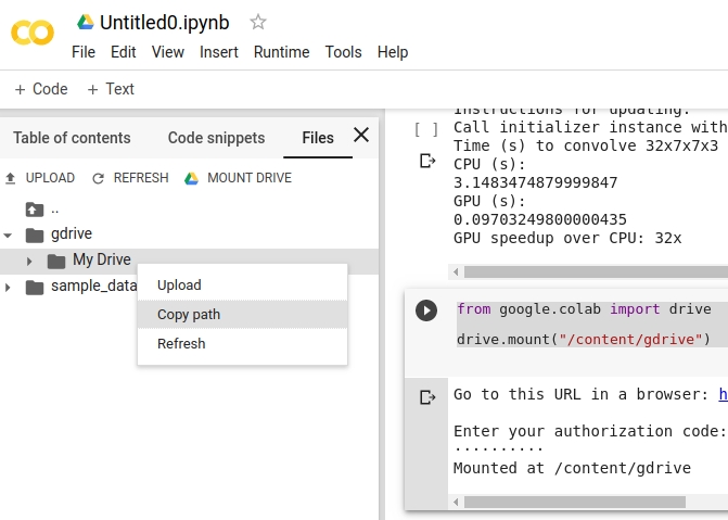 this copied text is the path of your HOME on Google Drive:
/content/gdrive/My Drive
from tensorflow.keras.models import Sequential
from tensorflow.keras.layers import Dense, Dropout, Activation, Flatten
from tensorflow.keras.layers import Conv2D, MaxPooling2D
from tensorflow.keras.callbacks import TensorBoard
from tensorflow.keras.utils import to_categorical
import pickle
import time
MODEL_NAME = "3-conv-128-layer-dense-1-out-2-softmax-categorical-cross-2-CNN"

pickle_in = open("/content/drive/My Drive/Projects/cat vs dog/Xv.pickle","rb")
X = pickle.load(pickle_in)

pickle_in = open("/content/drive/My Drive/Projects/cat vs dog/Y.pickle","rb")
y = pickle.load(pickle_in)
y = to_categorical(y)

X = X/255.0
model = Sequential()

model.add(Conv2D(128, (3, 3), input_shape=(50,50,1)))
model.add(Activation('relu'))
model.add(MaxPooling2D(pool_size=(2, 2)))
model.add(Dropout(0.3))

model.add(Conv2D(128, (3, 3)))
model.add(Activation('relu'))
model.add(MaxPooling2D(pool_size=(2, 2)))
model.add(Dropout(0.3))

model.add(Conv2D(128, (3, 3)))
model.add(Activation('relu'))
model.add(MaxPooling2D(pool_size=(2, 2)))
model.add(Dropout(0.3))

model.add(Flatten())

model.add(Dense(128))
model.add(Activation('relu'))

model.add(Dense(2))
model.add(Activation('softmax'))

tensorboard = TensorBoard(log_dir="/content/gdrive/My Drive/Colab/Logs/{}".format(MODEL_NAME))

model.compile(loss='categorical_crossentropy',
              optimizer='adam',
              metrics=['accuracy'],
              )

model.fit(X, y,
          batch_size=32,
          epochs=10,
          validation_split=0.3,
          callbacks=[tensorboard])
3.4 Classifying movie reviews: a binary classification example
In this example, you’ll learn to classify movie reviews as positive or negative, based on the text content of the reviews.3.4.1 The IMDB dataset
The IMDB dataset comes packaged with Keras. It has already been preprocessed:- the reviews (sequences of words) have been turned into sequences of integers, where each integer stands for a specific word in a dictionary.
- words are indexed by overall frequency in the dataset, so that for instance the integer "3" encodes the 3rd most frequent word in the data.
- "0" does not stand for a specific word, but instead is used to encode any unknown word.
from keras.datasets import imdb

(train_data, train_labels), (test_data, test_labels) = imdb.load_data(num_words=10000)
- The argument num_words=10000 means you’ll only keep the top 10,000 most frequently occurring words in the training data.
- The variables train_data and test_data are lists of reviews Each review is a list of word indices (encoding a sequence of words)
- train_labels and test_labels are lists of 0s and 1s 0 stands for negative and 1 stands for positive
word_index = imdb.get_word_index()
index_word = dict( [ (value, key) for (key, value) in word_index.items() ] )
decoded_review = ' '.join( [ index_word.get(i - 3, '?') for i in train_data[0] ] )
- imdb.get_word_index() Download the dictionary mapping from Downloading data from https://s3.amazonaws.com/text-datasets/imdb_word_index.json then return a dictionary where key are words (str) and values are indexes (integer). For ex., word_index["giraffe"] might return 1234.
- index_word is a dictionary mapping integer indices to words
- Note that the indices are offset by 3 because 0, 1, and 2 are reserved indices for “padding,” “start of sequence,” and “unknown.”
train_data[0][1]
14
index_word.get(14-3)
'this'
shoes=["adidas","ascis","nike"]
print('-'.join(shoes))

adidas-ascis-nike
3.4.2 Preparing the data
Each review is a list of word indices. We can’t feed lists of integers into a neural network which needs numerical values.One-hot encode your lists to turn them into vectors of 0s and 1s.
For instance, turning the sequence [3, 5] into a 10,000-dimensional vector that would be all 0s except for indices 3 and 5, which would be 1s.
import numpy as np

# data is a list of list:
# the 1st axix is the sample index,
# the 2nd axix is the review
def vectorize_sequences(sequences, dimension=10000):
    #Creates an all-zero matrix of shape (len(sequences), dimension)
    results = np.zeros((len(sequences), dimension))
    for i, sequence in enumerate(sequences):
        results[i, sequence] = 1.
    return results

x_train = vectorize_sequences(train_data)
x_test = vectorize_sequences(test_data)
It allows us to loop over something and have an automatic counter.
for counter, list_value in enumerate(some_list):
    print(counter, list_value)
If a word's index occurs in a sentence, it is coded 1.
The for loop use each review as the Boolean mask to encode the count of each word.
You should also vectorize your labels:
y_train = np.asarray(train_labels).astype('float32')
y_test = np.asarray(test_labels).astype('float32')
NumPy provides an N-dimensional array type, the ndarray, which describes a collection of “items” of the same type.
All ndarrays are homogenous: every item takes up the same size block of memory, and all blocks are interpreted in exactly the same way.
- numpy.asarray(a, dtype=None, order=None) Convert the input to an NumPy array. NumPy 裡面的 Array 與 Python 原生 List 不同,他是固定大小的,不像 Python List 可以動態增減。
- ndarray.astype(dtype, order='K', casting='unsafe', subok=True, copy=True) Copy of the array, cast to a specified type. NumPy 所有元件都需要是相同大小的,如此才能在記憶體有相同的 Size。
3.4.3 Building your network
keras.layers.Dense(units, activation=None, use_bias=True, kernel_initializer='glorot_uniform', bias_initializer='zeros', kernel_regularizer=None, bias_regularizer=None, activity_regularizer=None, kernel_constraint=None, bias_constraint=None)
- units Positive integer, dimensionality of the output space. (the same as the number of hidden units in this layer)
- activation Activation function to use. If you don't specify anything, no activation is applied (ie. "linear" activation: a(x) = x). Networks with a linear activation function are effectively only one layer deep, regardless of how complicated their architecture is. Real world and real problems are nonlinear . To make the incoming data non linear we use non linear mapping called activation function .
output = activation(dot(input, kernel) + bias)
- activation is the element-wise activation function passed as the activation argument
- kernel is a weights matrix created by the layer
- bias is a bias vector created by the layer (only applicable if use_bias is True)
Dense(16, activation='relu')16 is the number of hidden units of the layer.
Having 16 hidden units means the weight matrix W will have shape (input_dimension, 16), the dot product with W will project the input data onto a 16-dimensional representation space(and then you’ll add the bias vector b and apply the relu operation).
Having more hidden units allows your network to learn more-complex representations, but it makes the network more computationally expensive and may lead to learning unwanted patterns (patterns that will improve performance on the training data but not on the test data).
Therefore, there are two key architecture decisions to be made about such a stack of Dense layers:
- How many layers to use
- How many hidden units to choose for each layer
- Two intermediate layers with 16 hidden units each The intermediate layers will use relu as their activation function
- A third layer that will output the scalar prediction regarding the sentiment of the current review The final layer will use a sigmoid activation so as to output a probability (a score between 0 and 1, indicating how likely the sample is to have the target “1”(positive)
You can create a Sequential model by passing a list of layer instances to the constructor.
Here’s the Keras implementation,
from keras import models
from keras import layers

model = models.Sequential()
model.add(layers.Dense(16, activation='relu', input_shape=(10000,)))
model.add(layers.Dense(16, activation='relu'))
model.add(layers.Dense(1, activation='sigmoid'))
- An optimizer. This could be the string identifier of an existing optimizer (such as rmsprop or adagrad), or an instance of the Optimizer class.
- A loss function. This is the objective that the model will try to minimize. It can be the string identifier of an existing loss function (such as categorical_crossentropy or mse), or it can be an objective function.
- A list of metrics. For any classification problem you will want to set this to metrics=['accuracy']. A metric could be the string identifier of an existing metric or a custom metric function.
Here’s the step to configure the model with the rmsprop optimizer and the binary_crossentropy loss function.
model.compile(optimizer='rmsprop',
                      loss='binary_crossentropy',
                      metrics=['accuracy'])
3.4.4 Validating your approach
Keras models are trained on Numpy arrays of input data and labels. For training a model, you will typically use the fit function.
In order to monitor the accuracy of the model on data it has never seen(been trained) before during training, you’ll create a validation set by setting apart 10,000 samples from the original training data.
# data to be used to train the model
partial_x_train = x_train[10000:]
partial_y_train = y_train[10000:]

# data to be used to evaluate the model during the training
x_val = x_train[:10000]
y_val = y_train[:10000]
You’ll now train the model for 20 epochs (20 iterations over all samples in the x_train and y_train tensors), in mini-batches of 512 samples.
At the same time, you’ll monitor loss and accuracy on the 10,000 samples that you set apart. You do so by passing the validation data as the validation_data argument.
history = model.fit(partial_x_train, partial_y_train,
                    epochs=20,
                    batch_size=512,
                    validation_data=(x_val, y_val))
Train on 15000 samples, validate on 10000 samples
Epoch 1/20
15000/15000 [==============================] - 6s 394us/step - loss: 0.5084 - acc: 0.7813 - val_loss: 0.3797 - val_acc: 0.8684
...
Epoch 20/20
15000/15000 [==============================] - 3s 188us/step - loss: 0.0041 - acc: 0.9999 - val_loss: 0.6941 - val_acc: 0.8658
Note that the call to model.fit() returns a History object which has a member history.
It is a dictionary contains four entries: one per metric that was being monitored during training and during validation.
Let’s use Matplotlib to plot the training and validation loss side by side
import matplotlib.pyplot as plt
history_dict = history.history
loss_values = history_dict['loss']
val_loss_values = history_dict['val_loss']
acc = history_dict['acc']
epochs = range(1, len(acc) + 1)
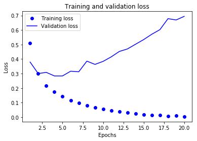
plt.plot(epochs, loss_values, 'bo', label='Training loss') # “bo” is for “blue dot.”
plt.plot(epochs, val_loss_values, 'b', label='Validation loss') # “b” is for “solid blue line.”
plt.title('Training and validation loss')
plt.xlabel('Epochs')
plt.ylabel('Loss')
plt.legend()
plt.show()
To plot the accuracy:
plt.clf() #Clears the figure

acc_values = history_dict['acc']
val_acc_values = history_dict['val_acc']
plt.plot(epochs, acc, 'bo', label='Training acc')
plt.plot(epochs, val_acc_values, 'b', label='Validation acc')
plt.title('Training and validation accuracy')
plt.xlabel('Epochs')
plt.ylabel('Loss')
plt.legend()
plt.show()()
plt.show()
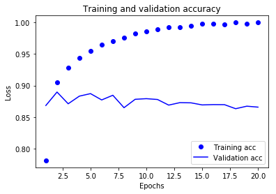
As you can see, the training loss decreases with every epoch, and the training accuracy increases with every epoch.
But that isn’t the case for the validation loss and accuracy: the validation loss is increased and the validation accuracy is decreased after the 5-th epoch.
This is overfitting: after the 2nd epoch, you’re overoptimizing on the training data.
In this case, to prevent overfitting, you could stop training earlier after 5 epochs.
model = models.Sequential()
model.add(layers.Dense(16, activation='relu', input_shape=(10000,)))
model.add(layers.Dense(16, activation='relu'))
model.add(layers.Dense(1, activation='sigmoid'))
model.compile(optimizer='rmsprop',
              loss='binary_crossentropy',
              metrics=['accuracy'])
model.fit(x_train, y_train, epochs=5, batch_size=512)
results = model.evaluate(x_test, y_test)
results

Out[29]:
[0.31565191437244416, 0.87944]
model.evaluate(x=None, y=None, batch_size=None, verbose=1, sample_weight=None, steps=None, callbacks=None, max_queue_size=10, workers=1, use_multiprocessing=False)

  Returns the loss value and metrics values for the model in test mode.
- x: Input data
- y: Target data
- batch_size: Integer or None.
- verbose: 0 or 1.
3.4.5 Using a trained network to generate predictions on new data
You can generate the likelihood of reviews being positive by using the predict method:
model.predict(x_test)

array([[ 0.1981305 ],
       [ 0.99992895],
       [ 0.72518015],
       ...,
       [ 0.12744974],
       [ 0.05118057],
       [ 0.70532745]], dtype=float32)
but less confident for others (0.6, 0.4).
3.4.6 Further experiments
3.4.7 Wrapping up
- You usually need to do quite a bit of preprocessing on your raw data in order to be able to feed it—as tensors—into a neural network.
- Stacks of Dense layers with relu activations can solve a wide range of problems (including sentiment classification)
- In a binary classification problem (two output classes), your network should end with a Dense layer with one unit and a sigmoid activation: the output of your network should be a scalar between 0 and 1, encoding a probability. With such a scalar sigmoid output on a binary classification problem, the loss function you should use is binary_crossentropy.
- The rmsprop optimizer is generally a good enough choice, whatever your problem.
- To avoid the overfitting, be sure to always monitor performance on data that is outside of the training set.
3.5 Classifying newswires: a multiclass classification example
In this section, you’ll build a network to classify Reuters newswires into 46 mutually exclusive topics.
The Reuters dataset is a set of short newswires and their topics, published by Reuters in 1986. It’s a simple, widely used toy dataset for text classification. There are 46 different topics.
the Reuters dataset comes packaged as part of Keras.
from keras.datasets import reuters

(train_data, train_labels), (test_data, test_labels) = reuters.load_data(
    num_words=10000)

>>> len(train_data)
8982
>>> len(test_data)
2246
Here’s how you can decode train_data[0] back to words,
word_index = reuters.get_word_index()
index_word = dict([(value, key) for (key, value) in word_index.items()])
decoded_newswire = ' '.join([index_word.get(i - 3, '?') for i in train_data[0]])
3.5.2 Preparing the data
Each short news is a list of word indices.
We need to encode the data in a value
import numpy as np

def vectorize_sequences(sequences, dimension=10000):
    results = np.zeros( (len(sequences), dimension) )
    for i, sequence in enumerate(sequences):
        results[i, sequence] = 1.
    return results

x_train = vectorize_sequences(train_data)
x_test = vectorize_sequences(test_data)

x_train.shape
(8982, 10000)
x_test.shape
(2246, 10000)
There are some methods to use the one-hot encoding of the labels: each label as an all-zero vector with a 1 in the place of the label index.
- a built-in way to do this in Keras
from keras.utils.np_utils import to_categorical

one_hot_train_labels = to_categorical(train_labels)
one_hot_test_labels = to_categorical(test_labels)
def to_one_hot(labels, dimension=46):
    results = np.zeros( (len(labels), dimension) )
    for i, label in enumerate(labels):
        results[i, label] = 1.
    return results

one_hot_train_labels = to_one_hot(train_labels)
one_hot_test_labels = to_one_hot(test_labels
3.5.3 Building your network
In the previous example, you used 16-dimensional intermediate layers, but a 16-dimensional space may be too limited to learn to separate 46 different classes: such small layers may act as information bottlenecks, therefore, let’s go with 64 units.
from keras import models
from keras import layers

model = models.Sequential()
model.add(layers.Dense(64, activation='relu', input_shape=(10000,)))
model.add(layers.Dense(64, activation='relu'))
model.add(layers.Dense(46, activation='softmax'))
- You end the network with a Dense layer of size 46 The network will output a 46-dimensional vector.
- The last layer uses a softmax activation. For every input sample, the network will produce a 46- dimensional output vector, where output[i] is the probability that the sample belongs to class i. The 46 scores will sum to 1.
model.compile(optimizer='rmsprop',
              loss='categorical_crossentropy',
              metrics=['accuracy'])
3.5.4 Validating your approach
# Set validation set
x_val = x_train[:1000]
y_val = one_hot_train_labels[:1000]
# Set trained set
partial_x_train = x_train[1000:]
partial_y_train = one_hot_train_labels[1000:]

# train the network for 20 epochs.
history = model.fit(partial_x_train,
                    partial_y_train,
                    epochs=20,
                    batch_size=512,
                    validation_data=(x_val, y_val))
import matplotlib.pyplot as plt
loss = history.history['loss']
val_loss = history.history['val_loss']
epochs = range(1, len(loss) + 1)
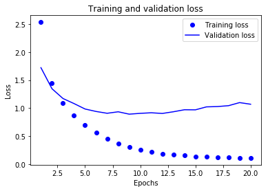
plt.plot(epochs, loss, 'bo', label='Training loss')
plt.plot(epochs, val_loss, 'b', label='Validation loss')
plt.title('Training and validation loss')
plt.xlabel('Epochs')
plt.ylabel('Loss')
plt.legend()
plt.show()
Plotting the training and validation accuracy
# Clears the figure
plt.clf()

acc = history.history['acc']
val_acc = history.history['val_acc']
plt.plot(epochs, acc, 'bo', label='Training acc')
plt.plot(epochs, val_acc, 'b', label='Validation acc')
plt.title('Training and validation accuracy')
plt.xlabel('Epochs')
plt.ylabel('Accuracy')
plt.legend()
plt.show()
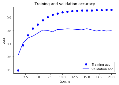
The network begins to overfit after 6-th epoch.
Let’s train a new network from scratch for 6 epochs and then evaluate it on the test set.
model = models.Sequential()
model.add(layers.Dense(64, activation='relu', input_shape=(10000,)))
model.add(layers.Dense(64, activation='relu'))
model.add(layers.Dense(46, activation='softmax'))
model.compile(optimizer='rmsprop',
              loss='categorical_crossentropy',
              metrics=['accuracy'])
model.fit(partial_x_train,
          partial_y_train,
          epochs=6,
          batch_size=512,
          validation_data=(x_val, y_val))
test_loss, test_accu = model.evaluate(x_test, one_hot_test_labels)
test_loss, test_accu
(0.99986814900582532, 0.77649154056954994)
3.5.5 Generating predictions on new data
predictions = model.predict(x_test)

predictions.shape # 2246 test inputs, each with 46 possible outcomes
(2246, 46)

np.sum(predictions[0]) #  the sum of the probability of all outcomes for the 1st input
1.0

np.argmax(predictions[0]) #  the class with the highest probability for the 1st imput
3

predictions[0][3] # the probability of the most possible outcome
0.74235409
3.5.6 A different way to handle the labels and the loss
If integer labels are used, you should use sparse_categorical_ crossentropy:
model.compile(optimizer='rmsprop', loss='sparse_categorical_crossentropy', metrics=['acc'])
3.5.7 The importance of having sufficiently large intermediate layers
You will introduce an information bottleneck by having intermediate layers that are significantly less than the input's dimensions.
The validation accuracy will have a significant drop. This drop is mostly due to the fact that you’re trying to compress a lot of information into an intermediate space that is too low-dimensional.
3.5.8 Further experiments
3.5.9 Wrapping up
3.6 Predicting house prices: a regression example
To predict a continuous value instead of a discrete label problem is called regression.
For instance, predicting the temperature tomorrow.
3.6.1 The Boston Housing Price dataset
The dataset has relatively few data points: only 506, split between 404 training samples and 102 test samples. And each feature in the input data (for example, the crime rate) has a different scale.
To load the Boston housing dataset
from keras.datasets import boston_housing

(train_data, train_targets), (test_data, test_targets) = boston_housing.load_data()

train_data.shape
(404, 13) # 404 training samples, 13 features
test_data.shape
(102, 13) # 102 test samples, 13 features
train_targets # the median values of owner-occupied homes ( in thousands of dollars)
[ 15.2,  42.3,  50. ...  19.4,  19.4,  29.1]
3.6.2 Preparing the data
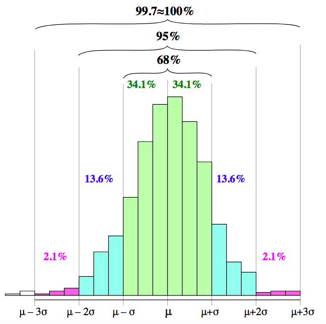
A widespread best practice to deal with data having wildly different ranges is to do do feature-wise normalization: for each feature in the input data (a column in the input data matrix), you subtract the mean of the feature and divide by the standard deviation, so that the feature's distribution is centered around 0 and has a unit standard deviation.
(x - Mean) / Standard Deviation
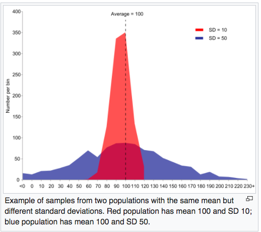
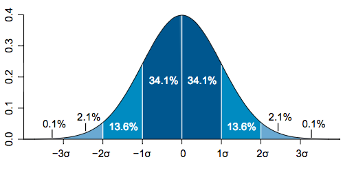
the 68–95–99.7 rule is a shorthand used to remember the percentage of values
把一個資料看成是一個樣本空間上的一點, 資料的n個feature就對應到n維空間上的每個座標上.
在樣本空間上,所有點座標其分量都相等的點(u, u, u, ...)所成的集合可被視為通過原點的對角線. 2維空間有2條對角線, 3維空間有3條對角線.
標準差可以被視為一個從n維空間的一個點到一條直線的距離的函數.
mean = train_data.mean(axis=0)
std = train_data.std(axis=0)

train_data -= mean
train_data /= std
test_data -= mean
test_data /= std
>>> print(results)
[[0. 0. 0. 0.]
 [1. 1. 1. 0.]
 [0. 0. 0. 0.]]
>>> results.mean(axis=0)
array([0.33333333, 0.33333333, 0.33333333, 0.        ])
>>> results.mean(axis=1)
array([0.  , 0.75, 0.  ])
3.6.3 Building your network
In general, the less training data you have, the worse overfitting will be, and using a small network is one way to mitigate overfitting.We use a very small network with two hidden layers, each with 64 units.
from keras import models
from keras import layers

# you use a function to construct it so that you can instantiate the same model multiple times
def build_model():
    model = models.Sequential()
    model.add(layers.Dense(64, activation='relu',
                            input_shape=(train_data.shape[1],)))
    model.add(layers.Dense(64, activation='relu'))
    model.add(layers.Dense(1))
    model.compile(optimizer='rmsprop', loss='mse', metrics=['mae'])
    return model
- The network ends with a single unit and no activation (it will be a linear layer). This is a typical setup for scalar regression (a regression where you’re trying to predict a single continuous value).
- the mse (mean squared error) loss function is used
- metric used for monitoring during training is mean absolute error (MAE)
3.6.4 Validating your approach using K-fold validation
The validation scores might have a high variance with regard to the validation split because the data points are too few.The best practice in such situations is to use K-fold cross-validation. ( sometimes called rotation estimation )
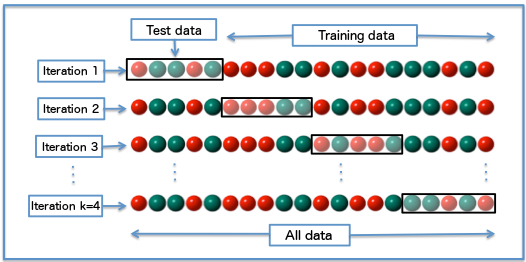
One of the main reasons for using cross-validation instead of using the conventional validation (e.g. partitioning the data set into two sets of 70% for training and 30% for test) is that there is not enough data available to partition it into separate training and test sets without losing significant modelling or testing capability.
It consists of:
- splitting the available data into K partitions
- instantiating K identical models, and training each one on K – 1 partitions while evaluating on the remaining partition
- The validation score for the model used is then the average of the K validation scores
import numpy as np
k=4
num_val_samples = int( len(train_data) / k )
num_epochs = 100
all_scores = []

for i in range(k):
    # Prepares the validation data: data from partition #k
    val_data = train_data[i * num_val_samples: (i + 1) * num_val_samples]
    val_targets = train_targets[i * num_val_samples: (i + 1) * num_val_samples]
    # Prepares the training data: data from all other partitions
    if ( i==0 ):
        partial_train_data = train_data[num_val_samples:]
        partial_train_targets = train_targets[num_val_samples:]
    else:
        partial_train_data = np.concatenate(
            [train_data[:i * num_val_samples],
            train_data[(i + 1) * num_val_samples:]], axis=0)
        partial_train_targets = np.concatenate( [train_targets[:i * num_val_samples],
            train_targets[(i + 1) * num_val_samples:]], axis=0)
    # Builds the Keras model (already compiled)
    model = build_model()
    # Trains the model ( in silent mode, verbose=0 )
    history = model.fit(partial_train_data, partial_train_targets,
       validation_data=(val_data, val_targets),
       epochs=num_epochs, batch_size=1, verbose=0)
    val_mse, val_mae = model.evaluate(val_data, val_targets, verbose=0)
    all_scores.append(val_mae)
numpy.concatenate( (a1, a2, ...), axis=0, out=None):
  Join a sequence of arrays along an existing axis.
The results:
>>> all_scores
[2.1638144738603344, 2.8611690266297596, 2.552104407017774, 2.3926332126749625]

>>> np.mean(all_scores)
2.4924302800457077
Let’s try training the network a bit longer: 500 epochs.
num_epochs = 500
all_mae_histories = []
for i in range(k):
    print('processing fold #', i, '/', k)
    # Prepare the validation data: data from partition #i
    val_data = train_data[i * num_val_samples: (i + 1) * num_val_samples]
    val_targets = train_targets[i * num_val_samples: (i + 1) * num_val_samples]
    # Prepares the training data: data from all other partitions
    if ( i==0 ):
        partial_train_data = train_data[num_val_samples:]
        partial_train_targets = train_targets[num_val_samples:]
    else:
        partial_train_data = np.concatenate(
            [train_data[:i * num_val_samples],
            train_data[(i + 1) * num_val_samples:]], axis=0)
        partial_train_targets = np.concatenate( [train_targets[:i * num_val_samples],
            train_targets[(i + 1) * num_val_samples:]], axis=0)
    print(len(val_data), len(partial_train_data))
    # Builds the Keras model (already compiled)
    model = build_model()
    # Trains the model ( in silent mode, verbose=0 )
    history = model.fit(partial_train_data, partial_train_targets,
       validation_data=(val_data, val_targets),
       epochs=num_epochs, batch_size=1, verbose=0)
    mae_history = history.history['val_mean_absolute_error']
    all_mae_histories.append(mae_history)

type(all_mae_histories)
list
len(all_mae_histories)
4
len(all_mae_histories[0])
500
average_mae_history = [
    np.mean([x[i] for x in all_mae_histories]) for i in range(num_epochs)]
import matplotlib.pyplot as plt
plt.plot(range(1, len(average_mae_history) + 1), average_mae_history)
plt.xlabel('Epochs')
plt.ylabel('Validation MAE')
plt.show()
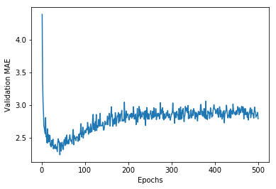
It may be a little difficult to see the plot, due to scaling issues and relatively high variance.
We can find the minimum MAE of each data fold and correspond indexes:
for i in range(4):
    print( all_mae_histories[i].index( min(all_mae_histories[i]) ),':', min(all_mae_histories[i]) )


32 : 1.81601905823
41 : 2.20111931433
39 : 2.3219555581
51 : 2.347481907
Therefore, the minimum happened before 51 epochs. Past that point, you start overfitting.
We can train a final production model on all of the training data, with the best parameters, and then look at its performance on the test data.
model = build_model()
model.fit(train_data, train_targets, epochs=60, batch_size=16, verbose=0)
test_mse_score, test_mae_score = model.evaluate(test_data, test_targets)

test_mae_score
2.8500603601044299
3.6.5 Wrapping up
- Mean squared error (MSE) is a loss function commonly used for regression.
- A common regression metric is mean absolute error (MAE).
- When features in the input data have values in different ranges, each feature should be scaled independently as a preprocessing step.
- When there is little data available, using K-fold validation is a great way to reliably evaluate a model.
- When little training data is available, it’s preferable to use a small network with few hidden layers (typically only one or two), in order to avoid severe overfitting.
4 Fundamentals of machine learning
4.1 Four branches of machine learning
4.1.1 Supervised learning
It consists of learning to map input data to known targets.4.1.2 Unsupervised learning
It consists of finding interesting transformations of the input data without the help of any targets.4.1.3 Self-supervised learning
It is supervised learning without any humans in the loop.
It's a kind of learning based on previous input.
4.1.4 Reinforcement learning
An agent receives information about its environment and learns to choose actions that will maximize some reward.4.2 Evaluating machine-learning models
The data is splitted into a training set, a validation set, and a test set.4.2.1 Training, validation, and test sets
You train on the training data and evaluate your model on the validation data. Once your model is ready for prime time, you test it one final time on the test data.Why is the validation set necessary? The reason is that developing a model always involves tuning its configuration: for example, choosing the number of layers or the size of the layers(called the hyper-parameters of the model).
In essence, this tuning is a form of learning: a search for a good configuration in some parameter space.
You’ll end up with a model that performs artificially well on the validation data, so you need to use a completely different, never-before-seen dataset to evaluate the model: the test dataset.
Your model shouldn’t have had access to any information about the test set, even indirectly.
Let’s review three classic evaluation recipes,
- simple hold-out validation
#
num_validation_samples = 10000
# Shuffling the data is usually appropriate
np.random.shuffle(data)

# Defines the validation set
validation_data = data[:num_validation_samples]
# Defines the training set
data = data[num_validation_samples:]
training_data = data[:]

model = get_model()
model.train(training_data)                         # train the model on the training set
validation_score = model.evaluate(validation_data) # and evaluates it on the validation set

# At this point you can tune your model,
# retrain it, evaluate it, tune it again...
model = get_model()
# to train your final model from scratch on all non-test data available.
model.train( np.concatenate( [training_data, validation_data] ) )
test_score = model.evaluate(test_data)
4.3 Data preprocessing, feature engineering, and feature learning
4.3.1 Data preprocessing for neural networks
- vectorization you must first turn all inputs into tensors of integers, a step called data vectorization. For ex., to represent a sentence as a list of integer index of words.
- normalization Take relatively large values can trigger large gradient updates that will prevent the network from converging. To make learning easier for your network, your data should have the following characteristics:
- small ranges — Typically, most values should be in the 0 ~ 1 range.
- homogenous — That is, all features should take values in roughly the same range.
x -= x.mean(axis=0) # Normalize each feature independently to have a mean of 0
x /= x.std(axis=0)  # Normalize each feature independently to have a standard deviation of 1.
4.3.2 Feature engineering
Feature engineering is the process of using your own knowledge about the input data and transform the input to be the data which can make the machine-learning algorithm work better by applying hardcoded (nonlearned) transformations to the data before it goes into the model.
4.4 Overfitting and underfitting
The fundamental issue in machine learning is the tension between optimization and generalization.
A model trained on more data will naturally generalize better.
If a network can only afford to memorize a small number of patterns, the optimization process will force it to focus on the most prominent patterns, which have a better chance of generalizing well.
4.4.1 Reducing the network’s size
Unfortunately, there is no magical formula to determine the right number of layers or the right size for each layer.The general workflow to find an appropriate model size is to start with relatively few layers and parameters, and increase the size of the layers or add new layers until you see diminishing returns with regard to validation loss.
4.4.2 Adding weight regularization
奥卡姆剃刀(英语:Occam's Razor, Ockham's Razor)是一個解決問題的法則. 同一個問題有許多種理論,若每一種都能做出同樣的預測,那麼應該挑選裡面假設最少的。
This idea also applies to the models learned by neural networks: given some training data and a network architecture, multiple sets of weight values (multiple models) could explain the data. Simpler models are less likely to overfit than complex ones.
A common way to mitigate overfitting is to put constraints on the complexity of a network by forcing its weights to take only small values, which makes the distribution of weight values more regular. This is called weight regularization, and it’s done by adding to the loss function of the network a cost associated with having large weights. This cost comes in two flavors:
- L1 regularization—The cost added is proportional to the absolute value of the weight coefficients (the L1 norm of the weights).
- L2 regularization—The cost added is proportional to the square of the value of the weight coefficients (the L2 norm of the weights).
from keras import regularizers

model = models.Sequential()
# Adding L2 weight regularization to the model
# l2(0.001) means every coefficient in the weight matrix of the layer will add
# 0.001 * weight_coefficient_value to the total loss of the network.
model.add(layers.Dense(16, kernel_regularizer=regularizers.l2(0.001), activation='relu', input_shape=(10000,)))
model.add(layers.Dense(16, kernel_regularizer=regularizers.l2(0.001), activation='relu'))
model.add(layers.Dense(1, activation='sigmoid'))
4.4.3 Adding dropout
Dropout, applied to a layer, consists of randomly dropping out a number of output features(setting weight coefficients to zero) of the layer during training.
In Keras, you can introduce dropout in a network via the Dropout layer, which is applied to the output of the layer right before it:
model.add(layers.Dropout(0.5))
4.5 The universal workflow of machine learning
4.5.1 Defining the problem and assembling a dataset
- You can only learn to predict something if you have available training data.
- Identifying the problem's classification type(binary, multi-class, regression, etc) will guide your choice of model architecture, loss function, and so on.
- Make sure your outputs can be predicted given your inputs.
4.5.2 Choosing a measure of success
Your metric for success will guide the choice of a loss function: what your model will optimize.
4.5.3 Deciding on an evaluation protocol
You must establish how you’ll measure your current progress during the training.
4.5.4 Preparing your data
You should format your data in a way that can be fed into a machine-learning model.
4.5.5 Developing a model that does better than a baseline
Choosing the right last-layer activation and loss function for your model:
| Problem type | Last-layer activation | Loss function |
|---|---|---|
| Binary classification | sigmoid | binary_crossentropy |
| Multiclass, single-label classification | softmax | categorical_crossentropy |
| Multiclass, multilabel classification | sigmoid | binary_crossentropy |
| Regression to arbitrary values | None | mse |
| Regression to values between 0 and 1 | sigmoid | mse or binary_crossentropy |
4.5.6 Scaling up: developing a model that overfits
Always monitor the training loss and validation loss, as well as the training and validation values for any metrics you care about. When you see that the model’s performance on the validation data begins to degrade, you’ve achieved overfitting.
4.5.7
Regularizing your model and tuning your hyperparameters
PART 2 Deep Learning in Practice
5 Deep learning for computer vision
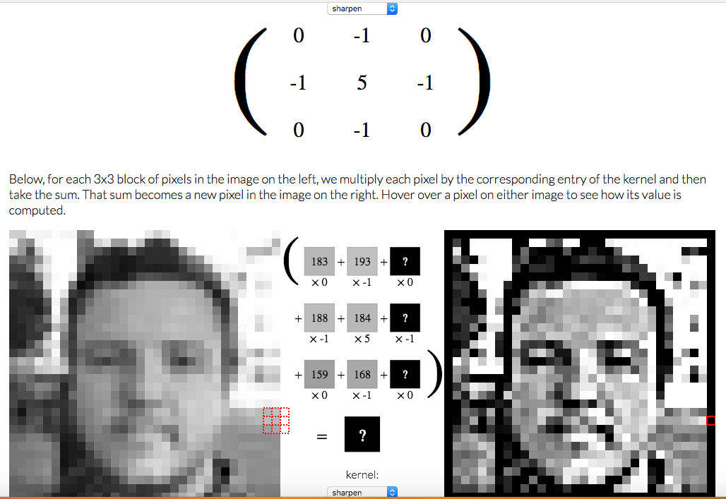
Convolution is the process of adding each element of the image to its local neighbors, weighted by the kernel.
The output of image convolution is calculated as follows:
- Place the kernel anchor on top of a determined pixel, with the rest of the kernel overlaying the corresponding local pixels in the image.
- Multiply the kernel coefficients by the corresponding image pixel values and sum the result.
- Place the result to the location of the anchor in the input image.
- Repeat the process for all pixels by scanning the kernel over the entire image.
An image kernel is a small matrix used in machine learning for feature extraction, a technique for determining the most important portions of an image.
The process is referred to more generally as "convolution".
The convolutional neural networks is also known as convnets.
Convolutional neural networks (CNNs) are the current state-of-the-art model architecture for image classification tasks.
CNNs are very similar to ordinary Neural Networks from the previous chapter: they are made up of neurons that have learnable weights and biases.
The difference is that ConvNet architectures make the explicit assumption that the inputs are images.
Neural Networks receive an input (a single vector), and transform it through a series of hidden layers. Each hidden layer is made up of a set of neurons, where each neuron is fully connected to all neurons in the previous layer, and where neurons in a single layer function completely independently and do not share any connections. The last fully-connected layer is called the “output layer” and in classification settings it represents the class scores.
Regular Neural Nets don’t scale well to full images. (Jerry: it's because the input is arranged in 1 dimensional array )
For images are of size 32x32x3 (32 wide, 32 high, 3 color channels), a single fully-connected neuron in a first hidden layer of a regular Neural Network would have 32*32*3 = 3072 weights. More neurons need more parameters. Clearly, this full connectivity is wasteful and the huge number of parameters would quickly lead to overfitting.
Unlike a regular Neural Network, the layers of a ConvNet have neurons arranged in 3 dimensions: width, height, depth.
Every layer of a ConvNet transforms the 3D input volume to a 3D output volume of neuron activations.
A simple ConvNet for CIFAR-10 dataset( 60000 32x32 colour images in 10 classes ) classification could have the architecture:
- INPUT [32x32x3] will hold the raw pixel values of the image, in this case an image of width 32, height 32, and with three color channels R,G,B.
- CONV layer will compute the output of neurons that are connected to local regions in the input, each computing a dot product between their weights and a small region they are connected to in the input volume. This may result in volume such as [32x32x12] if we decided to use 12 filters.(extract out 12 features)
- RELU layer will apply an element-wise activation function, such as the max(0,x)max(0,x) thresholding at zero. This leaves the size of the volume unchanged ([32x32x12]).
- POOL layer will perform a downsampling operation along the spatial dimensions (width, height), resulting in volume such as [16x16x12].
- FC (i.e. fully-connected) layer will compute the class scores, resulting in volume of size [1x1x10], where each of the 10 numbers correspond to a class score, such as among the 10 categories of CIFAR-10. As with ordinary Neural Networks and as the name implies, each neuron in this layer will be connected to all the numbers in the previous volume.
The parameters in the CONV/FC layers will be trained with gradient descent so that the class scores that the ConvNet computes are consistent with the labels in the training set for each image.
The Conv layer is the core building block of a Convolutional Network that does most of the computational heavy lifting.
When training a convnet, we don’t know what the values for our kernels and therefore have to figure them out by learning them.
The CONV layer’s parameters consist of a set of learnable filters. Every filter is small spatially (along width and height), but extends through the full depth of the input volume.
During the forward pass, we slide (more precisely, convolve) each filter across the width and height of the input volume and compute dot products between the entries of the filter and the input at any position. As we slide the filter over the width and height of the input volume we will produce a 2-dimensional activation map that gives the responses of that filter at every spatial position.
Each filter will produce a separate 2-dimensional activation map. We will stack these activation maps along the depth dimension and produce the output volume.
An example input volume (e.g. a 32x32x3 CIFAR-10 image), there are 5 neurons along the depth, all looking at the same region in the input. Each neuron in the convolutional layer is connected only to a local region in the input volume spatially, but to the full depth (i.e. all color channels)
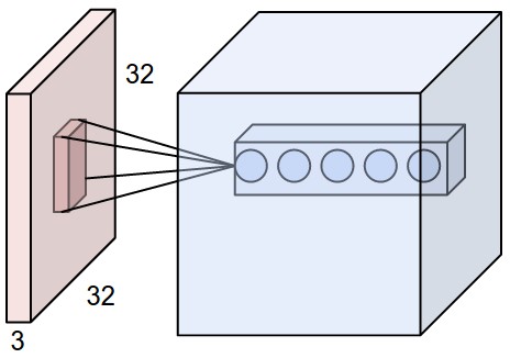
- Example 1 Suppose that the input volume has size [32x32x3]. If the receptive field (or the filter size) is 5x5, then each neuron in the Conv Layer will have weights to a [5x5x3] region in the input volume, for a total of 5*5*3 = 75 weights (and +1 bias parameter). Notice that the extent of the connectivity along the depth axis must be 3, since this is the depth of the input volume.
- Example 2 Suppose an input volume had size [16x16x20]. Then using an example receptive field size of 3x3, every neuron in the Conv Layer would now have a total of 3*3*20 = 180 connections to the input volume. Notice that, again, the connectivity is local in space (e.g. 3x3), but full along the input depth (20).
Three hyper-parameters control the size of the output volume: the depth, stride and zero-padding:
- the depth of the output volume it corresponds to the number of filters we would like to use, each learning to look for something different in the input. For example, if the first Convolutional Layer takes as input the raw image, then different neurons along the depth dimension may activate in presence of various oriented edges, or blobs of color. We will refer to a set of neurons that are all looking at the same region of the input as a depth column (some people also prefer the term fibre).
- the stride with which we slide the filter When the stride is 1 then we move the filters one pixel at a time. When the stride is 2 (or uncommonly 3 or more, though this is rare in practice) then the filters jump 2 pixels at a time as we slide them around. This will produce smaller output volumes spatially.
- pad the input volume with zeros around the border The size of this zero-padding is a hyperparameter. The nice feature of zero padding is that it will allow us to control the spatial size of the output volumes (most commonly as we’ll see soon we will use it to exactly preserve the spatial size of the input volume so the input and output width and height are the same).
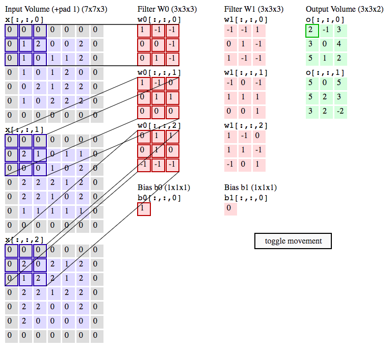
each output element is computed by element-wise multiplying the highlighted input (blue) with the filter (red), summing it up, and then offsetting the result by the bias.
o[0,0,0] = Conv( x[0, 0, 0], w0[0] ) +  Conv( x[0, 0, 0], w0[1] ) +  Conv( x[0, 0, 0], w0[2] )  + b0
         = -1 + 3 + (-1) + 1
         = 2
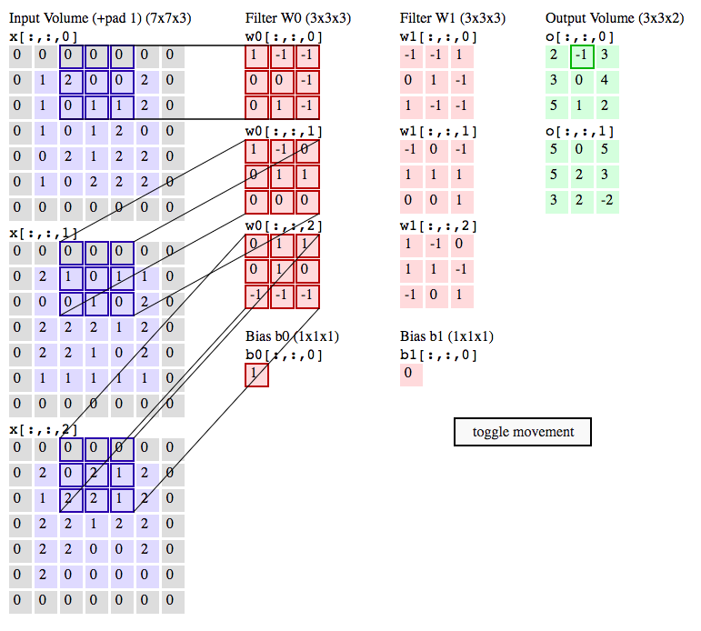
o[1,0,0] = Conv( x[2, 0, 0], w0[0] ) +  Conv( x[2, 0, 0], w0[1] ) +  Conv( x[2, 0, 0], w0[2] )  + b0
         = 0 + 1 + (-3) + 1
         = -1
Compare the regular 3-layer Neural Network with the CNN:
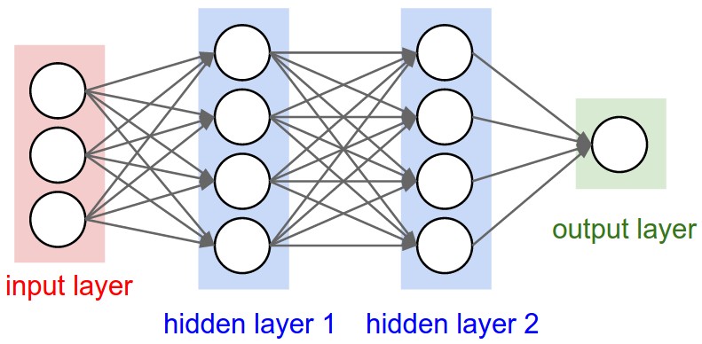 |  |
| Neurons are arranged in three dimensions. For RGB images, the depth is 3. |
5.1 Introduction to convnets
The most common form of a ConvNet architecture stacks a few CONV-RELU layers, follows them with POOL layers, and repeats this pattern until the image has been merged spatially to a small size. The last fully-connected layer holds the output, such as the class scores.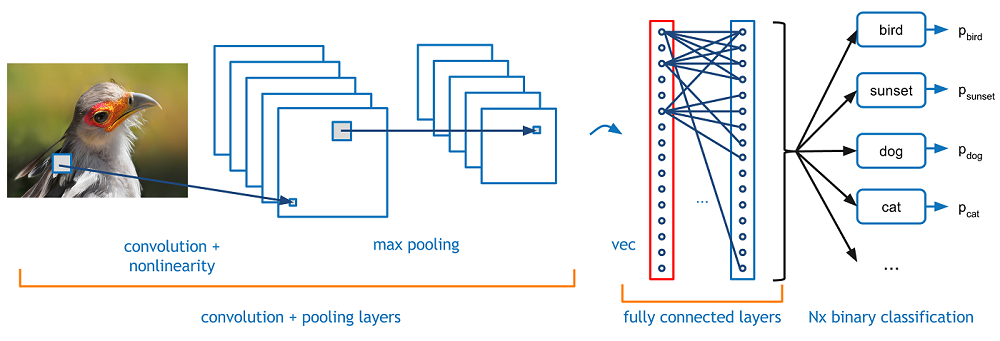
In other words, the most common ConvNet architecture follows the pattern:
INPUT -> [[CONV -> RELU]*N -> POOL?]*M -> [FC -> RELU]*K -> FC
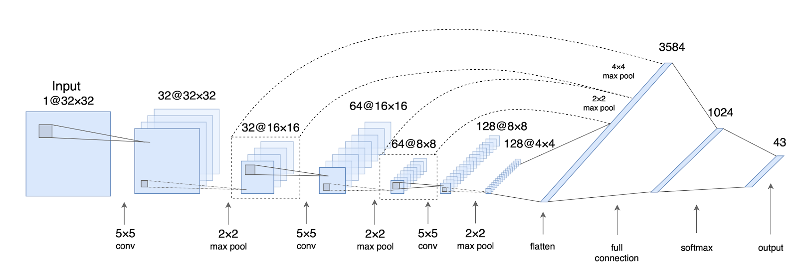
CNNs apply a series of filters(kernels/neurons) to the raw pixel data of an image to extract and learn higher-level features, which the model can then use for classification. CNNs contains three components:
- Convolutional layers which apply a specified number of convolution filters to the image. For each subregion(called the receptive field), the layer performs a set of mathematical operations to produce a single value in the output feature map.
- Pooling layers which downsample the image data extracted by the convolutional layers to reduce the dimensionality of the feature map in order to decrease processing time. A commonly used pooling algorithm is max pooling, which extracts subregions of the feature map (e.g., 2x2-pixel tiles), keeps their maximum value, and discards all other values.
- Dense (fully connected) layers which perform classification on the features extracted by the convolutional layers and downsampled by the pooling layers. In a dense layer, every node in the layer is connected to every node in the preceding layer.
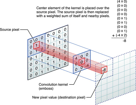 Convolutional layers then typically apply a ReLU activation function to the output to introduce nonlinearities into the model.
Typically, a CNN is composed of a stack of convolutional modules that perform feature extraction. Each module consists of a convolutional layer followed by a pooling layer. The last convolutional module is followed by one or more dense layers that perform classification. The final dense layer in a CNN contains a single node for each target class in the model (all the possible classes the model may predict), with a softmax activation function to generate a value between 0–1 for each node (the sum of all these softmax values is equal to 1). We can interpret the softmax values for a given image as relative measurements of how likely it is that the image falls into each target class.
from google.colab import drive
drive.mount("/content/gdrive")

# Instantiating a small convnet
from keras import layers
from keras import models

model = models.Sequential()
# process inputs of size (28, 28, 1)
model.add(layers.Conv2D(32, (3, 3), activation='relu', input_shape=(28, 28, 1)))
model.add(layers.MaxPooling2D((2, 2)))
model.add(layers.Conv2D(64, (3, 3), activation='relu'))
model.add(layers.MaxPooling2D((2, 2)))
model.add(layers.Conv2D(64, (3, 3), activation='relu'))

# Adding a classifier on top of the convnet,
# feed the last output tensor of the convnets into a densely connected classifier network
model.add(layers.Flatten())
# outputs are flattened into vectors of shape (576,) before going through two Dense layers.
model.add(layers.Dense(64, activation='relu'))
model.add(layers.Dense(10, activation='softmax'))

# Training the convnet on MNIST images
from keras.datasets import mnist
from keras.utils import to_categorical

# 載入內建的MNIST dataset
(train_images, train_labels), (test_images, test_labels) = mnist.load_data()

# reshape from (samples, width, height) into (samples, width, height, channels)
train_images = train_images.reshape((60000, 28, 28, 1))
# normalize
train_images = train_images.astype('float32') / 255

test_images = test_images.reshape((10000, 28, 28, 1))
test_images = test_images.astype('float32') / 255

train_labels = to_categorical(train_labels)
test_labels = to_categorical(test_labels)

model.compile(optimizer='rmsprop',
              loss='categorical_crossentropy',
              metrics=['accuracy'])
model.fit(train_images, train_labels, epochs=5, batch_size=64)

model.save(f"/content/gdrive/My Drive/Colab/Models/{MODEL_NAME}.model.hdf5")

test_loss, test_acc = model.evaluate(test_images, test_labels)

>>> test_acc
0.98960000000000004
- input_shape=(28, 28, 1) This is the format of MNIST image.
- every Conv2D and MaxPooling2D layer is a 3D tensor of shape (height, width, channels) The number of channels is controlled by the first argument passed to the Conv2D layers (32 or 64).
- the last output Dense layer is a classifier processing 1D vector We have to flatten the 3D outputs to 1D. keras.layers.Flatten() flattens the input. Does not affect the batch size. For ex.,
  # now: model.output_shape == (None, 64, 32, 32)
  model.add(Flatten())
  # now: model.output_shape == (None, 65536)
ndarray.astype(dtype) copy of the array then cast to a specified type.
keras.layers.Dense(units, activation) is the regular densely-connected Neural Network (hidden) layer where the number of neurons is assigned as units.
Dense implements the operation:
output = activation(dot(input, kernel) + bias)
- activation is the element-wise activation function passed as the activation argument,
- kernel is a weights matrix created by the layer, and
- bias is a bias vector created by the layer (only applicable if use_bias is True).
The saved model can be loaded for re-use:
from google.colab import drive
drive.mount("/content/gdrive")

# Instantiating a small convnet
from keras import layers
from keras import models
from keras.models import load_model

MODEL_NAME = "CNN-conv-32-64-64-maxpool-2-2-dense-64-10-relu-siftmax"

model = load_model(f"/content/gdrive/My Drive/Colab/Models/{MODEL_NAME}.model.hdf5")
# Training the convnet on MNIST images
from keras.datasets import mnist
from keras.utils import to_categorical

# 載入內建的MNIST dataset
(train_images, train_labels), (test_images, test_labels) = mnist.load_data()

# reshape from (samples, width, height) into (samples, width, height, channels)
train_images = train_images.reshape((60000, 28, 28, 1))
# normalize
train_images = train_images.astype('float32') / 255

test_images = test_images.reshape((10000, 28, 28, 1))
test_images = test_images.astype('float32') / 255

train_labels = to_categorical(train_labels)
test_labels = to_categorical(test_labels)
test_loss, test_acc = model.evaluate(test_images, test_labels)
5.1.1 The convolution operation
Dense layers learn global patterns in their input feature space (for example, for a MNIST digit, patterns involving all 28x28 pixels), whereas convolution layers learn local patterns. Images can be broken into local patterns such as edges, textures, and so on. Therefore, it's suitable to apply convnets to image-classification problems.This key characteristic gives convnets two interesting properties:
- The patterns they learn are translation invariant. After a pattern is learned, it can be identified independent of its location in the image.
- They can learn spatial hierarchies of patterns A first convolution layer will learn small local patterns such as edges, a second convolution layer will learn larger patterns made of the features of the first layers, and so on.
The convolution operation is a kind of filtering producing an output feature map.
Convolutions are defined by two key parameters:
- Size of the patches in the inputs to be operated
- Depth of the output feature map
keras.layers.Conv2D(filters, kernel_size, strides=(1, 1), padding='valid', data_format=None, dilation_rate=(1, 1), activation=None, use_bias=True, kernel_initializer='glorot_uniform', bias_initializer='zeros', kernel_regularizer=None, bias_regularizer=None, activity_regularizer=None, kernel_constraint=None, bias_constraint=None)
A convolution works by sliding kernel windows of size (window_height, window_width) over the 3D input. Each such 3D patch is then transformed (via a tensor product with the convolution kernel ) into a 1D vector of shape (output_depth,).
If the input is 5 x 5, there are only 9 tiles around which you can use a 3 × 3 window, forming a 3 × 3 grid. Hence, the output feature map will be 3 × 3. This is called the border effect. The following shows the 5x5 input and the 3x3 feature map:
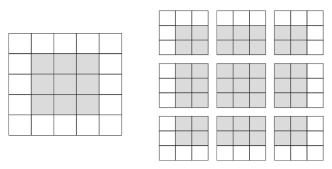
If you want to get an output feature map with the same spatial dimensions as the input, you can use padding.
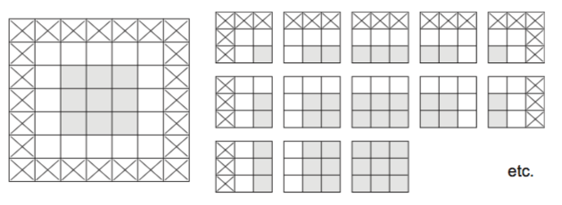
In Conv2D layers, padding is configurable via the padding argument:
- valid no padding (only valid window locations will be used). The default value.
- same pad in such a way as to have an output with the same width and height as the input
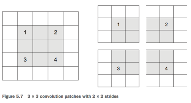
Strided convolutions are rarely used in practice, we tend to use the max-pooling operation.
model.summary()

_________________________________________________________________
Layer (type)                 Output Shape              Param #
=================================================================
conv2d_1 (Conv2D)            (None, 26, 26, 32)        320 = (3 x 3 + 1) x 32
_________________________________________________________________
max_pooling2d_1 (MaxPooling2 (None, 13, 13, 32)        0
_________________________________________________________________
conv2d_2 (Conv2D)            (None, 11, 11, 64)        18496 = ( 3 x 3 x 32 + 1 ) x 64
_________________________________________________________________
max_pooling2d_2 (MaxPooling2 (None, 5, 5, 64)          0
_________________________________________________________________
conv2d_3 (Conv2D)            (None, 3, 3, 64)          36928 = ( 3 x 3 x 64 + 1 ) x 64
_________________________________________________________________
flatten_1 (Flatten)          (None, 576)               0
_________________________________________________________________
dense_1 (Dense)              (None, 64)                36928 = (576 + 1) x 64
_________________________________________________________________
dense_2 (Dense)              (None, 10)                650 = (64 + 1) x 10
=================================================================
Total params: 93,322
Trainable params: 93,322
Non-trainable params: 0
  total_params =
    (filter_height * filter_width * input_image_channels + 1-bias ) * number_of_filters
Then, this feature map of size (26, 26, 32) is used as the input to the following max-pooling layer.
Convolutions are defined by two key parameters:
- Kernel size These are typically 3 × 3 or 5 × 5.
- Depth of the output feature map The number of filters(kernels).
5.1.2 The max-pooling operation
To summarize the output of a feature map, we can aggregate the values of a sub-matrix into a single value. One common way is the max-pooling which simply outputs the maximum activation value as observed in a region. An example of the max-pooling with the pool_size=(2,2):
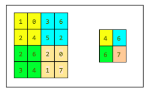
keras.layers.MaxPooling2D(pool_size=(2, 2), strides=None, padding='valid', data_format=None)
- pool_size integer or tuple of 2 integers, factors by which to downscale (vertical, horizontal). (2, 2) will halve the input in both spatial dimension. If only one integer is specified, the same window length will be used for both dimensions.
- strides Integer, tuple of 2 integers, or None. Strides values. If None, it will default to pool_size.
- padding One of "valid" or "same" (case-insensitive).
- data_format A string, one of channels_last (default) or channels_first. The ordering of the dimensions in the inputs. channels_last corresponds to inputs with shape (batch, height, width, channels) while channels_first corresponds to inputs with shape (batch, channels, height, width). "channels_last" is the default.
As the above example, the feature map of size (26, 26, 32) output by the 1st convolution layer is feed to the 2nd max-pooling layer (2,2) and the output is (13, 13, 32) .
5.2 Training a convnet from scratch on a small dataset
As a practical example, we’ll focus on classifying images as dogs or cats, in a dataset containing 4,000 pictures of cats and dogs (2,000 cats, 2,000 dogs). We’ll use 2,000 pictures for training—1,000 for validation, and 1,000 for testing. This will use three strategies:
- training a small model from scratch
- doing feature extraction using a pre-trained model
- fine-tuning a pre-trained model
5.2.1 The relevance of deep learning for small-data problems
There may be a lot of questions you had while reading:
- How do the filters in the first conv layer know to look for edges and curves?
- How does the fully connected layer know what activation maps to look at?
- How do the filters in each layer know what values to have?
5.2.2 Downloading the data
You can download the original dataset from www.kaggle.com/c/dogs-vs-cats/data
This dataset contains 25,000 images of dogs and cats (12,500 from each class) and is 543 MB (train.zip).
import os, shutil

original_dataset_dir = '/Users/jerry/.keras/datasets/kaggle_original_data/train'
base_dir = '/Users/jerry/.keras/datasets/cats_and_dogs_small'

os.mkdir(base_dir)
train_dir = os.path.join(base_dir, 'train')
os.mkdir(train_dir)
validation_dir = os.path.join(base_dir, 'validation')
os.mkdir(validation_dir)
test_dir = os.path.join(base_dir, 'test')
os.mkdir(test_dir)

train_cats_dir = os.path.join(train_dir, 'cats')
os.mkdir(train_cats_dir)
train_dogs_dir = os.path.join(train_dir, 'dogs')
os.mkdir(train_dogs_dir)
validation_cats_dir = os.path.join(validation_dir, 'cats')
os.mkdir(validation_cats_dir)
validation_dogs_dir = os.path.join(validation_dir, 'dogs')
os.mkdir(validation_dogs_dir)
test_cats_dir = os.path.join(test_dir, 'cats')
os.mkdir(test_cats_dir)
test_dogs_dir = os.path.join(test_dir, 'dogs')
os.mkdir(test_dogs_dir)

# Copies the first 1,000 cat images to train_cats_dir
fnames = ['cat.{}.jpg'.format(i) for i in range(1000)]
for fname in fnames:
    src = os.path.join(original_dataset_dir, fname)
    dst = os.path.join(train_cats_dir, fname)
    shutil.copyfile(src, dst)

# Copies the next 500 cat images to validation_cats_dir
fnames = ['cat.{}.jpg'.format(i) for i in range(1000, 1500)]
for fname in fnames:
    src = os.path.join(original_dataset_dir, fname)
    dst = os.path.join(validation_cats_dir, fname)
    shutil.copyfile(src, dst)

# Copies the next 500 cat images to test_cats_dir
fnames = ['cat.{}.jpg'.format(i) for i in range(1500, 2000)]
for fname in fnames:
    src = os.path.join(original_dataset_dir, fname)
    dst = os.path.join(test_cats_dir, fname)
    shutil.copyfile(src, dst)

# Copies the first 1,000 dog images to train_dogs_dir
fnames = ['dog.{}.jpg'.format(i) for i in range(1000)]
for fname in fnames:
    src = os.path.join(original_dataset_dir, fname)
    dst = os.path.join(train_dogs_dir, fname)
    shutil.copyfile(src, dst)

# Copies the next 500 dog images to validation_dogs_dir
fnames = ['dog.{}.jpg'.format(i) for i in range(1000, 1500)]
for fname in fnames:
    src = os.path.join(original_dataset_dir, fname)
    dst = os.path.join(validation_dogs_dir, fname)
    shutil.copyfile(src, dst)

# Copies the next 500 dog images to test_dogs_dir
fnames = ['dog.{}.jpg'.format(i) for i in range(1500, 2000)]
for fname in fnames:
    src = os.path.join(original_dataset_dir, fname)
    dst = os.path.join(test_dogs_dir, fname)
    shutil.copyfile(src, dst)

print('total training cat images:', len(os.listdir(train_cats_dir)))
print('total training dog images:', len(os.listdir(train_dogs_dir)))
print('total validation cat images:', len(os.listdir(validation_cats_dir)))
print('total validation dog images:', len(os.listdir(validation_dogs_dir)))
print('total test cat images:', len(os.listdir(test_cats_dir)))
print('total test dog images:', len(os.listdir(test_dogs_dir)))

total training cat images: 1000
total training dog images: 1000
total validation cat images: 500
total validation dog images: 500
total test cat images: 500
total test dog images: 500
The above uses Python's "list comprehensions". It can be used to construct lists in a very natural, easy way, like a mathematician is used to do.
S = {x² : x in {0 ... 9}}
V = (1, 2, 4, 8, ..., 2¹²)
M = {x | x in S and x even}
The above from mathematics can be implemented by Python:
>>> S = [x**2 for x in range(10)]
>>> V = [2**i for i in range(13)]
>>> M = [x for x in S if x % 2 == 0]
>>>
>>> print S; print V; print M
[0, 1, 4, 9, 16, 25, 36, 49, 64, 81]
[1, 2, 4, 8, 16, 32, 64, 128, 256, 512, 1024, 2048, 4096]
[0, 4, 16, 36, 64]
5.2.3 Building your network
In comparison with the MNIST datasets, we'll deal with bigger images and a more complex problem, we'll make the network larger : it will have one more Conv2D + MaxPooling2D stage.
# Instantiating a small convnet

from keras import layers
from keras import models

model = models.Sequential()
model.add(layers.Conv2D(32, (3, 3), activation='relu', input_shape=(150, 150, 3)))
model.add(layers.MaxPooling2D((2, 2)))
model.add(layers.Conv2D(64, (3, 3), activation='relu'))
model.add(layers.MaxPooling2D((2, 2)))
model.add(layers.Conv2D(128, (3, 3), activation='relu'))
model.add(layers.MaxPooling2D((2, 2)))
model.add(layers.Conv2D(128, (3, 3), activation='relu'))
model.add(layers.MaxPooling2D((2, 2)))
model.add(layers.Flatten())
model.add(layers.Dense(512, activation='relu'))
model.add(layers.Dense(1, activation='sigmoid')) # for a binary-classification problem
model.summary()
_________________________________________________________________
Layer (type)                 Output Shape              Param #
=================================================================
conv2d_4 (Conv2D)            (None, 148, 148, 32)      896
_________________________________________________________________
max_pooling2d_3 (MaxPooling2 (None, 74, 74, 32)        0
_________________________________________________________________
conv2d_5 (Conv2D)            (None, 72, 72, 64)        18496
_________________________________________________________________
max_pooling2d_4 (MaxPooling2 (None, 36, 36, 64)        0
_________________________________________________________________
conv2d_6 (Conv2D)            (None, 34, 34, 128)       73856
_________________________________________________________________
max_pooling2d_5 (MaxPooling2 (None, 17, 17, 128)       0
_________________________________________________________________
conv2d_7 (Conv2D)            (None, 15, 15, 128)       147584
_________________________________________________________________
max_pooling2d_6 (MaxPooling2 (None, 7, 7, 128)         0
_________________________________________________________________
flatten_2 (Flatten)          (None, 6272)              0
_________________________________________________________________
dense_3 (Dense)              (None, 512)               3211776
_________________________________________________________________
dense_4 (Dense)              (None, 1)                 513
=================================================================
Total params: 3,453,121
Trainable params: 3,453,121
Non-trainable params: 0

# Configuring the model for training

from keras import optimizers

model.compile( loss='binary_crossentropy', optimizer=optimizers.RMSprop(lr=1e-4), metrics=['acc'] )
5.2.4 Data preprocessing
Data should be formatted into appropriately preprocessed floating- point tensors before being fed into the network.
- Convert the pixel values into floating-point tensors.
- Rescale the pixel values (between 0 and 255) to the [0, 1] interval ( neural networks prefer to deal with small range input values).
Using the class ImageDataGenerator to read images from directories
from keras.preprocessing.image import ImageDataGenerator

# Rescales all images by 1/255
train_datagen = ImageDataGenerator(rescale=1./255)
test_datagen = ImageDataGenerator(rescale=1./255)

train_generator = train_datagen.flow_from_directory(
    train_dir, # Target directory
    target_size=(150, 150),  # Resizes all images to 150 × 150
    batch_size=20,
    class_mode='binary') #  you need binary labels for binary_crossentropy loss,
validation_generator = test_datagen.flow_from_directory(
    validation_dir,
    target_size=(150, 150),
    batch_size=20,
    class_mode='binary')

Found 2000 images belonging to 2 classes.
Found 1000 images belonging to 2 classes.
Generators are defined similar to function but there is only one difference, we use yield keyword to return value used for each iteration of the for loop. Let’s see an example where we are trying to clone python’s built-in range() function.
def my_range(start, stop, step = 1):
    if stop <= start:
        raise RuntimeError("start must be smaller than stop")
    i = start
    while i < stop:
        yield i
        i += step

try:
    for k in my_range(10, 50, 3):
        print(k)
except RuntimeError as ex:
    print(ex)
except:
    print("Unknown error occurred")
10
13
16
19
22
25
28
31
34
37
40
43
46
49
Yield are used in Python generators. A generator function is defined like a normal function, but whenever it needs to generate a value, it does so with the yield keyword rather than return. If the body of a def contains yield, the function automatically becomes a generator function.
keras.preprocessing.image.ImageDataGenerator(
featurewise_center=False, samplewise_center=False,
featurewise_std_normalization=False, samplewise_std_normalization=False,
zca_whitening=False, zca_epsilon=1e-06, rotation_range=0,
width_shift_range=0.0, height_shift_range=0.0,
brightness_range=None, shear_range=0.0, zoom_range=0.0,
channel_shift_range=0.0, fill_mode='nearest', cval=0.0,
horizontal_flip=False, vertical_flip=False, rescale=None, preprocessing_function=None,
data_format='channels_last', validation_split=0.0,
interpolation_order=1, dtype='float32')

ImageDataGenerator.flow_from_directory(
  directory, target_size=(256, 256), color_mode='rgb', classes=None,
  class_mode='categorical', batch_size=32, shuffle=True, seed=None,
  save_to_dir=None, save_prefix='', save_format='png', follow_links=False,
  subset=None, interpolation='nearest')
- directory path to the target directory. It should contain one subdirectory per class.
- target_size tuple of integers (height, width), default: (256, 256). The dimensions to which all images found will be resized.
- batch_size size of the batches of data (default: 32).
- classes Optional list of class subdirectories (e.g. ['dogs', 'cats']). Default: None. If not provided, the list of classes will be automatically inferred from the subdirectory names/structure under directory, where each subdirectory will be treated as a different class (and the order of the classes, which will map to the label indices, will be alphanumeric). The dictionary containing the mapping from class names to class indices can be obtained via the attribute class_indices.
- class_mode One of "categorical", "binary", "sparse", "input" or None. Default: "categorical". Determines the type of label arrays that are returned:
- categorical will be 2D one-hot encoded labels
- binary will be 1D binary labels
- sparse will be 1D integer labels
- input will be images identical to input images (mainly used to work with autoencoders).
- None, no labels are returned (the generator will only yield batches of image data, which is useful to use model.predict_generator(), model.evaluate_generator(), etc.). Please note that in case of class_mode None, the data still needs to reside in a subdirectory of directory for it to work correctly.
The fit_generator() method, the equivalent of fit() for data generators like this one. It expects as its first argument a Python generator that will yield batches of inputs and targets indefinitely.
The Keras model needs to know how many samples to draw from the generator before declaring an epoch over. This is the role of the steps_per_epoch argument: after having run for steps_per_epoch gradient descent steps — the fitting process will go to the next epoch.
Fitting the model using a batch generator:
history = model.fit_generator(
      train_generator,
      steps_per_epoch=100,
      epochs=30,
      validation_data=validation_generator,
      validation_steps=50)
- the architecture of the model, allowing to re-create the model
- the weights of the model
- the training configuration (loss, optimizer)
- the state of the optimizer, allowing to resume training exactly where you left off.
MODEL_NAME = "cats_and_dogs_small"

model.save(f"/content/gdrive/My Drive/Colab/Models/{MODEL_NAME}.model.hdf5")

from keras.models import load_model

model_2 = load_model(f"/content/gdrive/My Drive/Colab/Models/{MODEL_NAME}.model.hdf5")
import matplotlib.pyplot as plt
acc = history.history['acc']
val_acc = history.history['val_acc']
loss = history.history['loss']
val_loss = history.history['val_loss']
epochs = range(1, len(acc) + 1)
plt.plot(epochs, acc, 'bo', label='Training acc')
plt.plot(epochs, val_acc, 'b', label='Validation acc')
plt.title('Training and validation accuracy')
plt.legend()
plt.figure()
plt.plot(epochs, loss, 'bo', label='Training loss')
plt.plot(epochs, val_loss, 'b', label='Validation loss')
plt.title('Training and validation loss')
plt.legend()
plt.show()
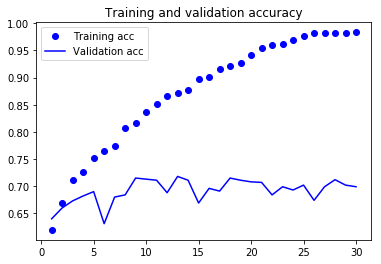
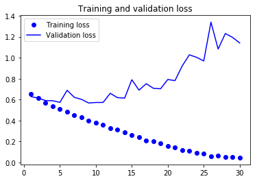
Because relatively few training samples (2,000) is used, overfitting( loss: validation > training ) will be the first concern.
5.2.5 Using data augmentation
Overfitting is caused by having too few samples to learn from, rendering you unable to train a model that can generalize to new data.
Data augmentation takes the approach of generating more training data from existing training samples, by augmenting the samples via a number of random transformations that yield believable-looking images.
In Keras, this can be done by configuring a number of random transformations to be performed on the images read by the ImageDataGenerator instance.
Setting up a data augmentation configuration via ImageDataGenerator:
datagen = ImageDataGenerator(
      rotation_range=40,
      width_shift_range=0.2,
      height_shift_range=0.2,
      shear_range=0.2,
      zoom_range=0.2,
      horizontal_flip=True,
      fill_mode='nearest')
The data will be looped over (in batches) indefinitely.
- rotation_range Int. Degree range for random rotations.
- width_shift_range Float (fraction of total width). Range for random horizontal shifts.
- height_shift_range Float (fraction of total height). Range for random vertical shifts.
- shear_range
Float. Shear Intensity (Shear angle in counter-clockwise direction as radians). - zoom_range Float or [lower, upper]. Range for random zoom. If a float, [lower, upper] = [1-zoom_range, 1+zoom_range].
- fill_mode One of {"constant", "nearest", "reflect" or "wrap"}. Points outside the boundaries(due to the transformations such as shift) of the input are filled according to the given mode:
- "constant" kkkkkkkk|abcd|kkkkkkkk (cval=k)
- "nearest" aaaaaaaa|abcd|dddddddd
- "reflect" abcddcba|abcd|dcbaabcd
- "wrap" abcdabcd|abcd|abcdabcd
- horizontal_flip Boolean. Randomly flip inputs horizontally.
 Shear is a transformation in which all points along a given line L remain fixed while other points are shifted parallel to L by a distance proportional to their perpendicular distance from L. Shearing a plane figure does not change its area.
Let’s look at the augmented images:
# Module with image preprocessing utilities
from keras.preprocessing import image

fnames = [os.path.join(train_cats_dir, fname) for fname in os.listdir(train_cats_dir)]
img_path = fnames[3] # Chooses one image to augment
img = image.load_img(img_path, target_size=(150, 150))  # Reads the image and resizes it

x = image.img_to_array(img) # Converts it to a Numpy array with shape (150, 150, 3)
# Reshapes it to (1, 150, 150, 3)
# because the flow() method requires the rank of 4
x = x.reshape( (1,) + x.shape )

# Generates batches of randomly transformed images.
import matplotlib.pyplot as plt

i=0
for batch in datagen.flow(x, batch_size=1):
    plt.figure(i)
    imgplot = plt.imshow(image.array_to_img(batch[0]))
    i += 1
    if i % 4 == 0:
        break  # Loops indefinitely, so you need to break the loop at some point!

plt.show()
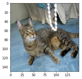
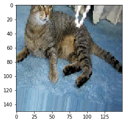
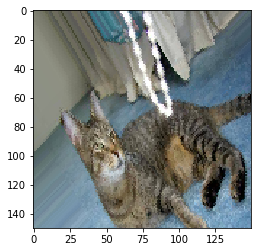
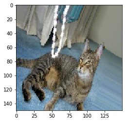
The method flow(x, y) takes numpy data and label arrays, and generates batches of augmented/normalized data.
Yields batches indefinitely, in an infinite loop.
- x Input data. Should have rank 4. In case of grayscale data, the channels axis should have value 1, and in case of RGB data, it should have value 3, and in case of RGBA data, it should have value 4.
- y labels
- batch_size int (default: 32).
But the inputs the network sees are still heavily intercorrelated, because they come from a small number of original images.
To further fight overfitting, you’ll also add a Dropout layer to your model, right before the densely connected classifier.
keras.layers.Dropout(rate, noise_shape=None, seed=None)
Dropout is a simple way to prevent neural networks from overfitting.
The key idea is to randomly drop units (along with their connections) from the neural network during training.
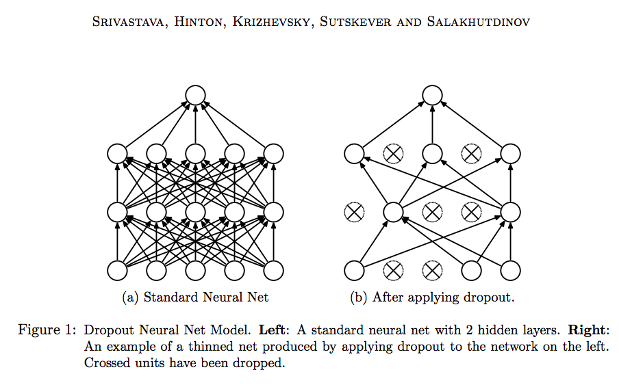
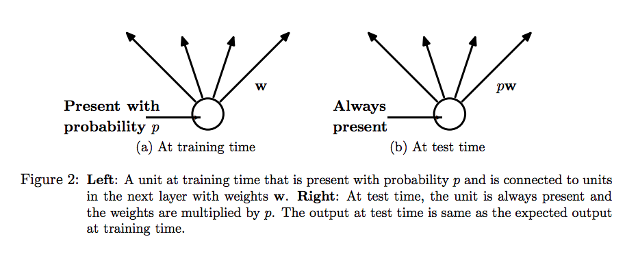
Dropout會讓每次batch run都依據機率丟棄一定比例的神經元不予計算,使得每一次都好像在訓練不同的神經網路一樣。
Defining a new convnet that includes dropout:
MODEL_NAME = "cats_and_dogs_small_dropout"

model = models.Sequential()
model.add(layers.Conv2D(32, (3, 3), activation='relu',
                        input_shape=(150, 150, 3)))
model.add(layers.MaxPooling2D((2, 2)))
model.add(layers.Conv2D(64, (3, 3), activation='relu'))
model.add(layers.MaxPooling2D((2, 2)))
model.add(layers.Conv2D(128, (3, 3), activation='relu'))
model.add(layers.MaxPooling2D((2, 2)))
model.add(layers.Conv2D(128, (3, 3), activation='relu'))
model.add(layers.MaxPooling2D((2, 2)))
model.add(layers.Flatten())
model.add(layers.Dropout(0.5))
model.add(layers.Dense(512, activation='relu'))
model.add(layers.Dense(1, activation='sigmoid'))
model.compile(loss='binary_crossentropy',
              optimizer=optimizers.RMSprop(lr=1e-4),
              metrics=['acc'])
Training the convnet using data-augmentation generators
train_datagen = ImageDataGenerator(
    rescale=1./255,
    rotation_range=40,
    width_shift_range=0.2,
    height_shift_range=0.2,
    shear_range=0.2,
    zoom_range=0.2,
    horizontal_flip=True,)
test_datagen = ImageDataGenerator(rescale=1./255)  # Note that the validation data shouldn’t be augmented!

train_generator = train_datagen.flow_from_directory(
        train_dir,                     # Target directory
        target_size=(150, 150),        # Resizes all images to 150 × 150
        batch_size=32,
        class_mode='binary')           # Because you use binary_crossentropy loss, you need binary labels.

validation_generator = test_datagen.flow_from_directory(
        validation_dir,
        target_size=(150, 150),
        batch_size=32,
        class_mode='binary')
history = model.fit_generator(
      train_generator,
      steps_per_epoch=100,
      epochs=50,
      validation_data=validation_generator,
      validation_steps=50)

# Saving the model
model.save(f"/content/gdrive/My Drive/Colab/Models/{MODEL_NAME}.model.hdf5")
Original model, Epoch 1/30 100/100 [==============================] - 149s 1s/step - loss: 0.6550 - acc: 0.6195 - val_loss: 0.6283 - val_acc: 0.6400 Epoch 2/30 100/100 [==============================] - 121s 1s/step - loss: 0.6152 - acc: 0.6695 - val_loss: 0.6142 - val_acc: 0.6600 Epoch 3/30 100/100 [==============================] - 120s 1s/step - loss: 0.5704 - acc: 0.7105 - val_loss: 0.5908 - val_acc: 0.6730 ... Epoch 30/30 100/100 [==============================] - 113s 1s/step - loss: 0.0469 - acc: 0.9835 - val_loss: 1.1403 - val_acc: 0.6990 |
Model with data augmentation and dropout, Epoch 1/30 100/100 [==============================] - 200s 2s/step - loss: 0.6896 - acc: 0.5381 - val_loss: 0.6748 - val_acc: 0.5571 Epoch 2/30 100/100 [==============================] - 196s 2s/step - loss: 0.6753 - acc: 0.5709 - val_loss: 0.6599 - val_acc: 0.5928 Epoch 3/30 100/100 [==============================] - 197s 2s/step - loss: 0.6622 - acc: 0.5850 - val_loss: 0.6311 - val_acc: 0.6332 ... Epoch 30/30 100/100 [==============================] - 199s 2s/step - loss: 0.4901 - acc: 0.7659 - val_loss: 0.4893 - val_acc: 0.7684 |
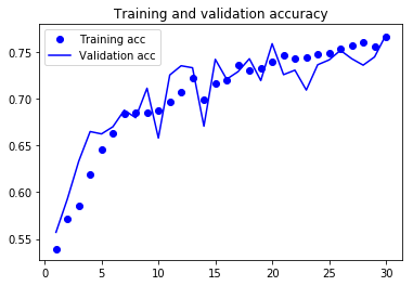
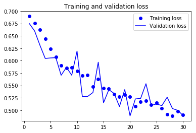
Thanks to data augmentation and dropout, you’re no longer overfitting: the training curves are closely tracking the validation curves. And, an accuracy of 7% relative improvement over the non-regularized model.
But it would prove difficult to go any higher because you have so little data to work with.
5.3 Using a pretrained convnet
A pretrained network is a saved network that was previously trained on a large dataset.
The VGG16 architecture was developed by Karen Simonyan and Andrew Zisserman in 2014; it’s a simple and widely used convnet architecture for ImageNet.
Its architecture is similar to what you’re already familiar with and is easy to understand without introducing any new concepts.
There are two ways to use a pretrained network: feature extraction and fine-tuning.
5.3.1 Feature extraction
Feature extraction consists of using the representations learned by a previous network to extract interesting features from new samples. These features are then run through a new classifier, which is trained from scratch.
The convnet used for image classification comprise two parts: they start with a series of convolution and pooling layers, and they end with a denselyconnected classifier.
The first part is called the convolutional base of the model.
The representations learned by the convolutional base are likely to be more generic and therefore more reusable.
Layers that come earlier in the model extract local, highly generic feature maps (such as visual edges, colors, and textures), whereas layers that are higher up extract more-abstract concepts (such as “cat ear” or “dog eye”).
Let’s put this in practice by using the convolutional base of the VGG16 network, trained on ImageNet, to extract interesting features from cat and dog images, and then train a dogs-versus-cats classifier on top of these features.
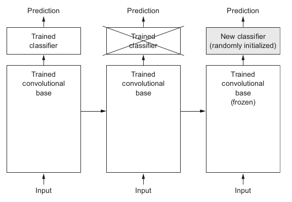
The VGG16 model, among others, comes prepackaged with Keras. You can import it from the keras.applications module.
Here’s the list of image-classification models (all pretrained on the ImageNet dataset) that are available as part of keras.applications:
- Xception
- Inception V3
- ResNet50
- VGG16
- VGG19
- MobileNet
from keras.applications import VGG16

conv_base_model = VGG16(weights='imagenet',
                  include_top=False,
                  input_shape=(150, 150, 3))
- weights one of None (random initialization) or 'imagenet' (pre-training on ImageNet).
- include_top whether to include the 3 fully-connected layers at the top of the network. By default, this densely connected classifier corresponds to the 1,000 classes from ImageNet. If you intend to use your own densely connected classifier, you don’t need to include it.
- input_shape optional shape tuple, only to be specified if include_top is False (otherwise the input shape has to be (224, 224, 3) (with 'channels_last' data format) or (3, 224, 224) (with 'channels_first' data format). It should have exactly 3 inputs channels, and width and height should be no smaller than 48. E.g. (200, 200, 3) would be one valid value.
Downloading data from https://github.com/fchollet/deep-learning-models/releases/download/v0.1/vgg16_weights_tf_dim_ordering_tf_kernels_notop.h5
58892288/58889256 [==============================] - 33s 1us/step
conv_base_model.summary()

_________________________________________________________________
Layer (type)                 Output Shape              Param #
=================================================================
input_2 (InputLayer)         (None, 150, 150, 3)       0
_________________________________________________________________
block1_conv1 (Conv2D)        (None, 150, 150, 64)      1792
_________________________________________________________________
block1_conv2 (Conv2D)        (None, 150, 150, 64)      36928
_________________________________________________________________
block1_pool (MaxPooling2D)   (None, 75, 75, 64)        0
_________________________________________________________________
block2_conv1 (Conv2D)        (None, 75, 75, 128)       73856
_________________________________________________________________
block2_conv2 (Conv2D)        (None, 75, 75, 128)       147584
_________________________________________________________________
block2_pool (MaxPooling2D)   (None, 37, 37, 128)       0
_________________________________________________________________
block3_conv1 (Conv2D)        (None, 37, 37, 256)       295168
_________________________________________________________________
block3_conv2 (Conv2D)        (None, 37, 37, 256)       590080
_________________________________________________________________
block3_conv3 (Conv2D)        (None, 37, 37, 256)       590080
_________________________________________________________________
block3_pool (MaxPooling2D)   (None, 18, 18, 256)       0
_________________________________________________________________
block4_conv1 (Conv2D)        (None, 18, 18, 512)       1180160
_________________________________________________________________
block4_conv2 (Conv2D)        (None, 18, 18, 512)       2359808
_________________________________________________________________
block4_conv3 (Conv2D)        (None, 18, 18, 512)       2359808
_________________________________________________________________
block4_pool (MaxPooling2D)   (None, 9, 9, 512)         0
_________________________________________________________________
block5_conv1 (Conv2D)        (None, 9, 9, 512)         2359808
_________________________________________________________________
block5_conv2 (Conv2D)        (None, 9, 9, 512)         2359808
_________________________________________________________________
block5_conv3 (Conv2D)        (None, 9, 9, 512)         2359808
_________________________________________________________________
block5_pool (MaxPooling2D)   (None, 4, 4, 512)         0
=================================================================
Total params: 14,714,688
Trainable params: 14,714,688
Non-trainable params: 0
- Recording its output to a Numpy array on disk, and then using this data as input to a standalone, densely connected classifier. This technique won’t allow you to use data augmentation.
Extracting features using the pretrained convolutional base:
The extracted features are currently of shape (samples, 4, 4, 512). You’ll feed them to a densely connected classifier, so first you must flatten themimport os import numpy as np from keras.preprocessing.image import ImageDataGenerator MODEL_NAME = "cats_and_dogs_small" base_dir = '/content/gdrive/My Drive/Colab/Datasets/cats_and_dogs_small' train_dir = os.path.join(base_dir, 'train') validation_dir = os.path.join(base_dir, 'validation') test_dir = os.path.join(base_dir, 'test') datagen = ImageDataGenerator(rescale=1./255) batch_size = 20 def extract_features(directory, sample_count): features = np.zeros(shape=(sample_count, 4, 4, 512)) labels = np.zeros(shape=(sample_count)) generator = datagen.flow_from_directory( directory, target_size=(150, 150), batch_size=batch_size, class_mode='binary') i=0 for inputs_batch, labels_batch in generator: features_batch = conv_base_model.predict(inputs_batch) features[i * batch_size : (i + 1) * batch_size] = features_batch labels[i * batch_size : (i + 1) * batch_size] = labels_batch i += 1 if i * batch_size >= sample_count: break # Note that because generators yield data indefinitely in a loop, you must break after every image has been seen once. return features, labels train_features, train_labels = extract_features(train_dir, 2000) validation_features, validation_labels = extract_features(validation_dir, 1000) test_features, test_labels = extract_features(test_dir, 1000)
Define your densely connected classifier and train it on the data and labels that you just recorded.train_features = np.reshape(train_features, (2000, 4 * 4 * 512)) validation_features = np.reshape(validation_features, (1000, 4 * 4 * 512)) test_features = np.reshape(test_features, (1000, 4 * 4 * 512))
This training and validation process is only for the fully connected layers.from keras import models from keras import layers from keras import optimizers model = models.Sequential() model.add(layers.Dense(256, activation='relu', input_dim=4 * 4 * 512)) model.add(layers.Dropout(0.5)) model.add(layers.Dense(1, activation='sigmoid')) model.compile(optimizer=optimizers.RMSprop(lr=2e-5), loss='binary_crossentropy', metrics=['acc']) history = model.fit(train_features, train_labels, epochs=30, batch_size=20, validation_data=(validation_features, validation_labels)) MODEL_NAME = "cats_and_dogs_small_vgg16_dense_dropout" model.save(f"/content/gdrive/My Drive/Colab/Models/{MODEL_NAME}.model.hdf5")
Let’s look at the loss and accuracy curves during trainingimport matplotlib.pyplot as plt acc = history.history['acc'] val_acc = history.history['val_acc'] loss = history.history['loss'] val_loss = history.history['val_loss'] epochs = range(1, len(acc) + 1) plt.plot(epochs, acc, 'bo', label='Training acc') plt.plot(epochs, val_acc, 'b', label='Validation acc') plt.title('Training and validation accuracy') plt.legend() plt.figure() plt.plot(epochs, loss, 'bo', label='Training loss') plt.plot(epochs, val_loss, 'b', label='Validation loss') plt.title('Training and validation loss') plt.legend() plt.show()

You reach a validation accuracy of about 90% — much better than you achieved with the small model trained from scratch. But the plots also indicate that you’re overfitting almost from the start — despite using dropout with a fairly large rate. That’s because this technique doesn’t use data augmentation, which is essential for preventing overfitting with small image datasets.
- Extending the current model you have ( conv_base_model ) by adding Dense layers on top. This technique is far more time expensive than the first, but which allows you to use data augmentation during training: extending the conv_base_model and running it end to end on the inputs. NOTE This technique is so expensive that you should only attempt it if you have access to a GPU.
from keras import models
from keras import layers
model = models.Sequential()
model.add(conv_base_model)
model.add(layers.Flatten())
model.add(layers.Dense(256, activation='relu'))
model.add(layers.Dense(1, activation='sigmoid'))
model.summary()
Model: "sequential_2" _________________________________________________________________ Layer (type) Output Shape Param # ================================================================= vgg16 (Model) (None, 4, 4, 512) 14714688 _________________________________________________________________ flatten_1 (Flatten) (None, 8192) 0 _________________________________________________________________ dense_3 (Dense) (None, 256) 2097408 _________________________________________________________________ dense_4 (Dense) (None, 1) 257 ================================================================= Total params: 16,812,353 Trainable params: 16,812,353 Non-trainable params: 0Before you compile and train the model, it’s very important to freeze the convolutional layers. Freezing a layer or set of layers means preventing their weights from being updated during training. In Keras, you freeze a network by setting its trainable attribute to False :
conv_base_model.trainable = False
from keras.preprocessing.image import ImageDataGenerator
from keras import optimizers
train_datagen = ImageDataGenerator(
rescale=1./255,
rotation_range=40,
width_shift_range=0.2,
height_shift_range=0.2,
shear_range=0.2,
zoom_range=0.2,
horizontal_flip=True,
fill_mode='nearest')
# Note that the validation data shouldn’t be augmented!
test_datagen = ImageDataGenerator(rescale=1./255)
train_generator = train_datagen.flow_from_directory(
train_dir,
target_size=(150, 150),
batch_size=20,
class_mode='binary')
validation_generator = test_datagen.flow_from_directory(
validation_dir,
target_size=(150, 150),
batch_size=20,
class_mode='binary')
model.compile(loss='binary_crossentropy',
optimizer=optimizers.RMSprop(lr=2e-5),
metrics=['acc'])
history = model.fit_generator(
train_generator,
steps_per_epoch=100,
epochs=30,
validation_data=validation_generator,
validation_steps=50)
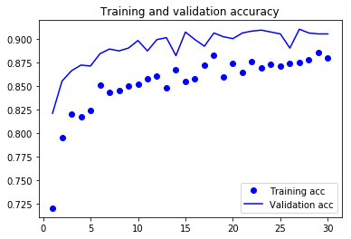
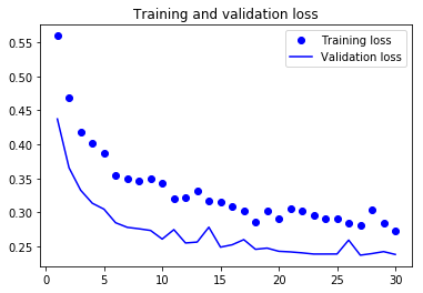
5.3.2 Fine-tuning
The steps for fine-tuning a network are as follow:- Add your custom network on top of an already-trained base network.
- Freeze the base network.
- Train the part you added.
- Unfreeze some layers in the base network.
- Jointly train both these layers and the part you added.
from keras.applications import VGG16
conv_base_model = VGG16(weights='imagenet',
include_top=False,
input_shape=(150, 150, 3))
>>> conv_base_model.summary()
Model: "vgg16" _________________________________________________________________ Layer (type) Output Shape Param # ================================================================= input_1 (InputLayer) (None, 150, 150, 3) 0 _________________________________________________________________ block1_conv1 (Conv2D) (None, 150, 150, 64) 1792 _________________________________________________________________ block1_conv2 (Conv2D) (None, 150, 150, 64) 36928 _________________________________________________________________ block1_pool (MaxPooling2D) (None, 75, 75, 64) 0 _________________________________________________________________ block2_conv1 (Conv2D) (None, 75, 75, 128) 73856 _________________________________________________________________ block2_conv2 (Conv2D) (None, 75, 75, 128) 147584 _________________________________________________________________ block2_pool (MaxPooling2D) (None, 37, 37, 128) 0 _________________________________________________________________ block3_conv1 (Conv2D) (None, 37, 37, 256) 295168 _________________________________________________________________ block3_conv2 (Conv2D) (None, 37, 37, 256) 590080 _________________________________________________________________ block3_conv3 (Conv2D) (None, 37, 37, 256) 590080 _________________________________________________________________ block3_pool (MaxPooling2D) (None, 18, 18, 256) 0 _________________________________________________________________ block4_conv1 (Conv2D) (None, 18, 18, 512) 1180160 _________________________________________________________________ block4_conv2 (Conv2D) (None, 18, 18, 512) 2359808 _________________________________________________________________ block4_conv3 (Conv2D) (None, 18, 18, 512) 2359808 _________________________________________________________________ block4_pool (MaxPooling2D) (None, 9, 9, 512) 0 _________________________________________________________________ block5_conv1 (Conv2D) (None, 9, 9, 512) 2359808 _________________________________________________________________ block5_conv2 (Conv2D) (None, 9, 9, 512) 2359808 _________________________________________________________________ block5_conv3 (Conv2D) (None, 9, 9, 512) 2359808 _________________________________________________________________ block5_pool (MaxPooling2D) (None, 4, 4, 512) 0 ================================================================= Total params: 14,714,688 Trainable params: 14,714,688 Non-trainable params: 0You’ll fine-tune the last three convolutional layers, which means all layers up to block4_pool should be frozen, and the layers block5_conv1 , block5_conv2 , and block5_conv3 should be trainable. Why not fine-tune more layers?
- Earlier layers in the convolutional base encode more-generic, reusable features
- The more parameters you’re training, the more you’re at risk of overfitting.
- Load the pre-trained VGG16 model
MODEL_NAME = "cats_and_dogs_small_vgg16_5.3.2"
from keras.applications import VGG16
conv_base_model = VGG16(weights='imagenet',
include_top=False,
input_shape=(150, 150, 3))
conv_base_model.trainable = True
set_trainable = False
for layer in conv_base_model.layers:
if layer.name == 'block5_conv1':
set_trainable = True
if set_trainable:
layer.trainable = True
else:
layer.trainable = False
from keras.preprocessing.image import ImageDataGenerator
from keras import optimizers
import os
import numpy as np
base_dir = '/content/gdrive/My Drive/Colab/Datasets/cats_and_dogs_small'
train_dir = os.path.join(base_dir, 'train')
validation_dir = os.path.join(base_dir, 'validation')
test_dir = os.path.join(base_dir, 'test')
train_datagen = ImageDataGenerator(
rescale=1./255,
rotation_range=40,
width_shift_range=0.2,
height_shift_range=0.2,
shear_range=0.2,
zoom_range=0.2,
horizontal_flip=True,
fill_mode='nearest')
# Note that the validation data shouldn’t be augmented!
test_datagen = ImageDataGenerator(rescale=1./255)
train_generator = train_datagen.flow_from_directory(
train_dir,
target_size=(150, 150),
batch_size=20,
class_mode='binary')
validation_generator = test_datagen.flow_from_directory(
validation_dir,
target_size=(150, 150),
batch_size=20,
class_mode='binary')
from keras import models
from keras import layers
model = models.Sequential()
model.add(conv_base_model)
model.add(layers.Flatten())
model.add(layers.Dense(256, activation='relu'))
model.add(layers.Dense(1, activation='sigmoid'))
model.compile(loss='binary_crossentropy',
optimizer=optimizers.RMSprop(lr=1e-5),
metrics=['acc'])
history = model.fit_generator(
train_generator,
steps_per_epoch=100,
epochs=30,
validation_data=validation_generator,
validation_steps=50)
MODEL_NAME = "cats_and_dogs_small_tuningConv_ext_dense"
model.save(f"/content/gdrive/My Drive/Colab/Models/{MODEL_NAME}.model.hdf5")
import matplotlib.pyplot as plt
acc = history.history['acc']
val_acc = history.history['val_acc']
loss = history.history['loss']
val_loss = history.history['val_loss']

epochs = range(1, len(acc) + 1)

plt.plot(epochs, acc, 'bo', label='Training acc')
plt.plot(epochs, val_acc, 'b', label='Validation acc')
plt.title('Training and validation accuracy')
plt.legend()
plt.figure()
plt.plot(epochs, loss, 'bo', label='Training loss')
plt.plot(epochs, val_loss, 'b', label='Validation loss')
plt.title('Training and validation loss')
plt.legend()
plt.show()
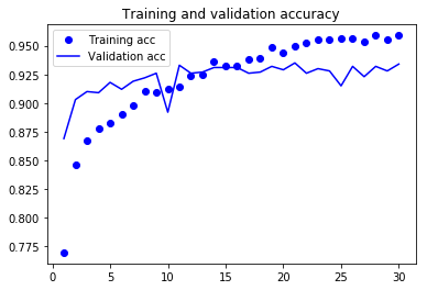
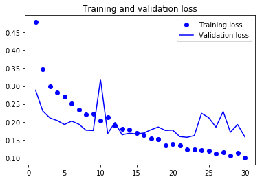 Note that the loss curve doesn’t show any real improvement. What you display is an average of pointwise loss values; but what matters for accuracy is the result of a binary thresholding of the class probability predicted by the model.
test_generator = test_datagen.flow_from_directory(
test_dir,
target_size=(150, 150),
batch_size=20,
class_mode='binary')
test_loss, test_acc = model.evaluate_generator(test_generator, steps=50)
print('test acc:', test_acc)
Found 1000 images belonging to 2 classes. test acc: 0.9419999945163727
5.4 Visualizing what convnets learn
The representations learned by convnets are representations of visual concepts which are present in a human-readable form.
Techniques have been developed for visualizing and interpreting these representations.
5.4.1 Visualizing intermediate activations
The output of a layer is often called its activation.
This gives a view into how an input is decomposed into the different filters learned by the network.
Let’s start by loading the model that you saved in section 5.2:
from keras.models import load_model
MODEL_NAME = "cats_and_dogs_small_30epoch"
model = load_model(f"/content/gdrive/My Drive/Colab/Models/{MODEL_NAME}.model.hdf5")
model.summary()
Model: "sequential_1" _________________________________________________________________ Layer (type) Output Shape Param # ================================================================= conv2d_1 (Conv2D) (None, 148, 148, 32) 896 _________________________________________________________________ max_pooling2d_1 (MaxPooling2 (None, 74, 74, 32) 0 _________________________________________________________________ conv2d_2 (Conv2D) (None, 72, 72, 64) 18496 _________________________________________________________________ max_pooling2d_2 (MaxPooling2 (None, 36, 36, 64) 0 _________________________________________________________________ conv2d_3 (Conv2D) (None, 34, 34, 128) 73856 _________________________________________________________________ max_pooling2d_3 (MaxPooling2 (None, 17, 17, 128) 0 _________________________________________________________________ conv2d_4 (Conv2D) (None, 15, 15, 128) 147584 _________________________________________________________________ max_pooling2d_4 (MaxPooling2 (None, 7, 7, 128) 0 _________________________________________________________________ flatten_1 (Flatten) (None, 6272) 0 _________________________________________________________________ dense_1 (Dense) (None, 512) 3211776 _________________________________________________________________ dense_2 (Dense) (None, 1) 513 ================================================================= Total params: 3,453,121 Trainable params: 3,453,121 Non-trainable params: 0
Preprocessing a single image from the test set:
img_path = '/content/gdrive/My Drive/Colab/Datasets/cats_and_dogs_small/test/cats/cat.1700.jpg'
from keras.preprocessing import image
import numpy as np
# Preprocesses the image into a 4D tensor
img = image.load_img(img_path, target_size=(150, 150))
img_tensor = image.img_to_array(img)
img_tensor = np.expand_dims(img_tensor, axis=0)
img_tensor /= 255.
print(img_tensor.shape)
(1, 150, 150, 3)
matplotlib.pyplot.imshow(X, cmap=None,...):
X : array-like or PIL image
The image data. Supported array shapes are:
*(M, N): an image with scalar data. The data is visualized using a colormap.
*(M, N, 3): an image with RGB values (0-1 float or 0-255 int).
*(M, N, 4): an image with RGBA values (0-1 float or 0-255 int), i.e. including transparency.
numpy.expand_dims(a, axis):
Expand the shape of an array.
Insert a new axis that will appear at the axis position in the expanded array shape.
Let’s display the picture:
import matplotlib.pyplot as plt
plt.imshow(img_tensor[0])
plt.show()
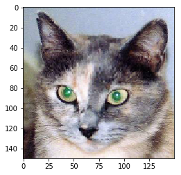
There are two main types of models available in Keras:
- the Sequential model
- the Model class used with the functional API
- model.layers is a flattened list of the layers comprising the model.
- model.inputs is the list of input tensors of the model.
- model.outputs is the list of output tensors of the model.
- model.summary() prints a summary representation of your model.
- model.get_config() returns a dictionary containing the configuration of the model.
In the functional API, given some input tensor(s) and output tensor(s), you can instantiate a Model via:
from keras.models import Model
from keras.layers import Input, Dense
a = Input(shape=(32,))
b = Dense(32)(a)
model = Model(inputs=a, outputs=b)
Instantiating a model:
from keras import models
# Extracts the outputs of the top eight layers
# Skip the Flatten and Dense layers
layer_outputs = [layer.output for layer in model.layers[:8]]
# Creates a model that will return these outputs, given the model input
model_activation = models.Model(inputs=model.input, outputs=layer_outputs)
activations = model_activation.predict(img_tensor)
len(activations)
8
activations[0].shape
(1, 148, 148, 32)
import matplotlib.pyplot as plt
first_layer_activation = activations[0]
plt.matshow(first_layer_activation[0, :, :, 4], cmap='viridis')
Display an array as a matrix in a new figure window.
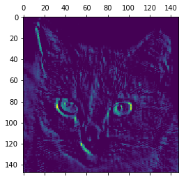
Let’s try the 7-th channel,
plt.matshow(first_layer_activation[0, :, :, 7], cmap='viridis')
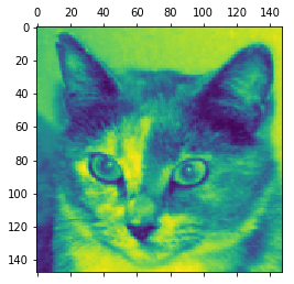
Let’s plot a complete visualization of all the activations in the network,
# Names of the layers, so you can have them as part of your plot
layer_names = []
for layer in model.layers[:8]:
layer_names.append(layer.name)
images_per_row = 16
for layer_name, layer_activation in zip(layer_names, activations):
# Number of features in the feature map ( 4D sensor )
n_features = layer_activation.shape[-1]
# The feature map has shape (1, size, size, n_features).
size = layer_activation.shape[1]
# Tiles the activation channels in this matrix
n_rows = n_features // images_per_row
display_grid = np.zeros((size * n_rows, images_per_row * size))
# Tiles each filter into a big horizontal grid
for row in range(n_rows):
for col in range(images_per_row):
channel_image = layer_activation[0,
:, :,
row * images_per_row + col]
# Post-processes the feature to make it visually palatable
channel_image -= channel_image.mean()
channel_image /= channel_image.std()
channel_image *= 64
channel_image += 128
channel_image = np.clip(channel_image, 0, 255).astype('uint8')
# Displays the grid
display_grid[row * size : (row + 1) * size,
col * size : (col + 1) * size] = channel_image
scale = 1. / size
plt.figure(figsize=(scale * display_grid.shape[1],
scale * display_grid.shape[0]))
plt.title(layer_name)
plt.grid(False)
plt.imshow(display_grid, aspect='auto', cmap='viridis')
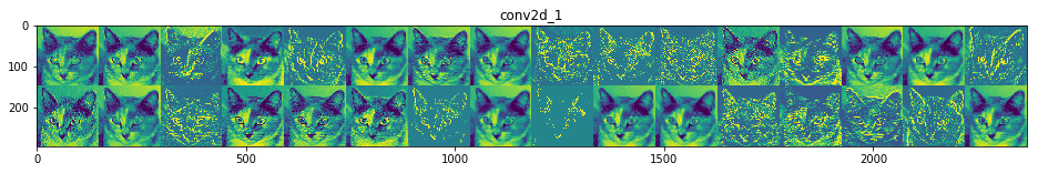
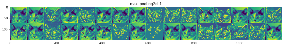
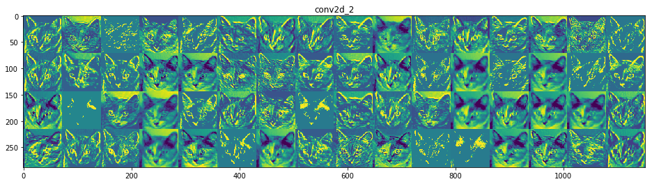
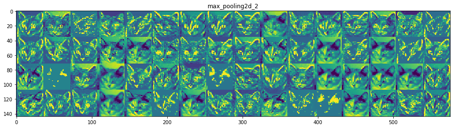
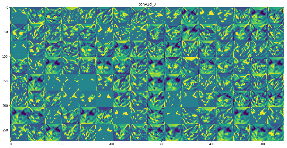
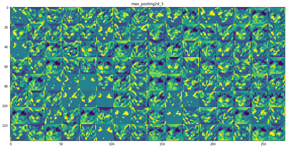
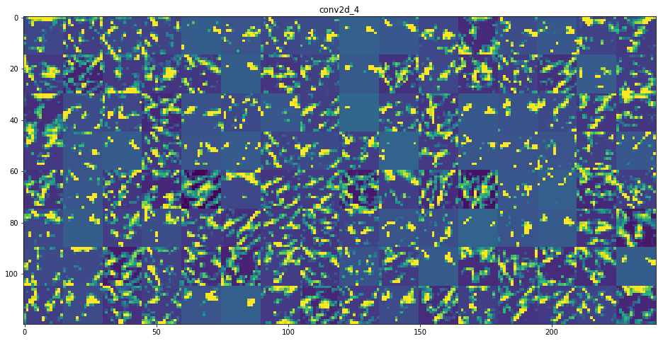
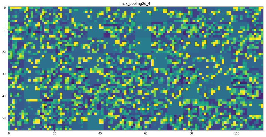
There are a few things to note here:
- Python zip() Function The zip() function returns a zip object, which is an iterator of tuples. Join two tuples together:
a = ("John", "Charles", "Mike")
b = ("Jenny", "Christy", "Monica")
x = zip(a, b)
#use the tuple() function to display a readable version of the result:
print(tuple(x))
(('John', 'Jenny'), ('Charles', 'Christy'), ('Mike', 'Monica'))
“cat eye.”)
You brain has learned to completely abstract its visual input—to transform it into high-level visual concepts while filtering out irrelevant visual details.
Some tasks, for instance, require multimodal inputs: they merge data coming from different input sources and each type of input data uses different kinds of neural layers.
5.4.2 Visualizing convnet filters
5.4.3 Visualizing heatmaps of class activation
6 Deep learning for text and sequences
6.1 Working with text data
Deep-learning models only work with numeric tensors. Vectorizing text is the process of transforming text into numeric tensors.
The different units into which you can break down text (words, characters, or n-grams) are called tokens, and breaking text into such tokens is called tokenization.
All text-vectorization processes consist of applying some tokenization scheme and then associating numeric vectors with the generated tokens.
There are two major tokenization scheme:
- one-hot encoding of tokens
- token embedding (typically used exclusively for words, and called word embedding).
" n-gram" 指文中連續出現的n個語詞。n-gram語法模型是基於(n-1)階馬爾可夫鏈的一種概率語言模型,通過n個語詞出現的概率來推斷語句的結構。
Word n-grams are groups of N (or fewer) consecutive words that you can extract from a sentence.
For ex., “The cat sat on the mat.”,
It may be decomposed into the following set of
- 2-grams
{"The", "The cat", "cat", "cat sat", "sat", "sat on",
"on", "on the", "the", "the mat", "mat"}
{"The", "The cat", "The cat sat","cat", "cat sat", "cat sat on",
"sat", "sat on", "sat on the", "on", "on the", , "on the mat",
"the", "the mat", "mat"}
Extracting n-grams is a form of feature engineering.6.1.1 One-hot encoding of words and characters
One-hot encoding consists of associating a unique integer index with every word and then turning this integer index i into a binary vector of size N (the size of the vocabulary); the vector is all zeros except for the i th entry, which is 1.
One example for character-level one-hot encoding:
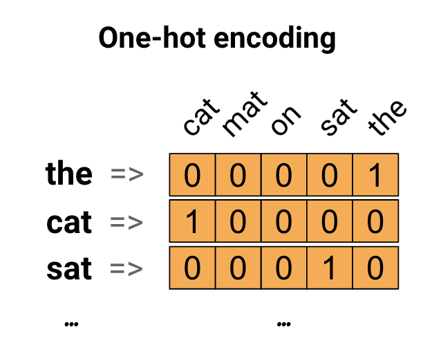
import string
samples = ['The cat sat on the mat.', 'The dog ate my homework.']
characters = string.printable # All printable ASCII
# ASCII char: index
ascii_table = dict(zip(characters, range(1, len(characters) + 1)))
max_length = 50
results = np.zeros( ( len(samples), max_length, max(ascii_table.values()) + 1 ) )
for i, sample in enumerate(samples):
for j, character in enumerate(sample):
index = ascii_table.get(character)
results[i, j, index] = 1
from keras.preprocessing.text import Tokenizer
samples = ['The cat sat on the mat.', 'The dog ate my homework.']
# Creates a tokenizer, configured to only take into account the 1,000 most common words
tokenizer = Tokenizer(num_words=1000)
# Builds the word index
tokenizer.fit_on_texts(samples)
# Turns strings into lists of integer indices
sequences = tokenizer.texts_to_sequences(samples)
# You could also directly get the one-hot binary representations.
# Vectorization modes other than one-hot encoding are supported by this tokenizer.
one_hot_results = tokenizer.texts_to_matrix(samples, mode='binary')
# How you can recover the word index that was computed
word_index = tokenizer.word_index
print('Found %s unique tokens.' % len(word_index))
- fit_on_texts(texts) texts: list of texts to train on.
- texts_to_sequences(texts) texts: list of texts to turn to sequences.
- texts_to_matrix(texts) texts: list of texts to vectorize. mode: one of "binary", "count", "tfidf", "freq" (default: "binary"). Return: numpy array of shape (len(texts), nb_words).
- word_index dictionary mapping words (str) to their rank/index (int). Only set after fit_on_texts was called.
tokenizer.word_docs
defaultdict(int,
{'ate': 1,
'cat': 1,
'dog': 1,
'homework': 1,
'mat': 1,
'my': 1,
'on': 1,
'sat': 1,
'the': 2})
tokenizer.word_index
{'ate': 7,
'cat': 2,
'dog': 6,
'homework': 9,
'mat': 5,
'my': 8,
'on': 4,
'sat': 3,
'the': 1}
sequences
[[1, 2, 3, 4, 1, 5], [1, 6, 7, 8, 9]]
one_hot_results.shape
(2, 1000)
one_hot_results[0][0:10]
array([0., 1., 1., 1., 1., 1., 0., 0., 0., 0.])
one_hot_results[1][0:10]
array([0., 1., 0., 0., 0., 0., 1., 1., 1., 1.])
| #0 | #1 | #2 | #3 | #4 | #5 | #6 | #7 | #8 | #9 | |
| NULL | the | cat | sat | on | mat | dog | ate | my | homework | |
6.1.2 Using word embeddings
One-hot encode your text will have tens of thousands of unique words in your text vocabulary.
Word embeddings map a set of words or phrases in a vocabulary to vectors of numerical values.
Word embeddings use an efficient dense representation in which similar words have a similar encoding.
An embedding is a dense vector of floating point values which are trainable parameters.
It is common to see word embeddings that are 8-dimensional (for small datasets), up to 1024-dimensions when working with large datasets. A higher dimensional embedding can capture fine-grained relationships between words, but takes more data to learn.
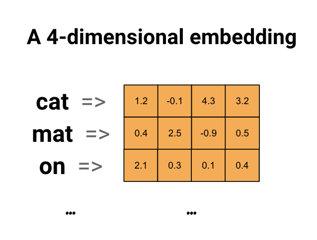
Above is a diagram for a word embedding. Each word is represented as a 4-dimensional vector of floating point values. Another way to think of an embedding is as "lookup table". After these weights have been learned, we can encode each word by looking up the dense vector it corresponds to in the table.
There are two ways to obtain word embeddings:
- Learning word embeddings with the embeddings layer To learn a new embedding space is about learning the weights of a layer: the Embedding layer. The Embedding layer can be understood as a lookup table that maps from integer indices (which stand for specific words) to dense vectors (their embeddings). Instantiating an Embedding layer:
from keras.layers import Embedding
embedding_layer = Embedding(1000, 64)
- input_dim Size of the vocabulary, i.e. maximum integer index + 1.
- output_dim Dimension of the dense embedding.
- Input shape 2D tensor with shape: (batch_size, sequence_length).
- Output shape 3D tensor with shape: (batch_size, sequence_length, output_dim).
- Loading the IMDB data for use with an Embedding layer
from keras.datasets import imdb
from keras import preprocessing
#restrict the movie reviews to the top 10,000 most common words(features)
max_features = 10000
# Cuts off the review to max 20 characters
maxlen = 20
#Loads the data as lists of integers
(x_train, y_train), (x_test, y_test) = imdb.load_data(num_words=max_features)
x_train = preprocessing.sequence.pad_sequences(x_train, maxlen=maxlen)
x_test = preprocessing.sequence.pad_sequences(x_test, maxlen=maxlen)
from keras.layers import Embedding
from keras.models import Sequential
from keras.layers import Flatten, Dense
model = Sequential()
model.add(Embedding(10000, 8, input_length=maxlen))
model.add(Flatten())
model.add(Dense(1, activation='sigmoid'))
model.compile(optimizer='rmsprop', loss='binary_crossentropy', metrics=['acc'])
model.summary()
Model: "sequential_2"
_________________________________________________________________
Layer (type) Output Shape Param #
=================================================================
embedding_1 (Embedding) (None, 20, 8) 80000
_________________________________________________________________
flatten_1 (Flatten) (None, 160) 0
_________________________________________________________________
dense_1 (Dense) (None, 1) 161
=================================================================
Total params: 80,161
Trainable params: 80,161
Non-trainable params: 0
history = model.fit(x_train, y_train,
epochs=10,
batch_size=32,
validation_split=0.2)
20000/20000 [==============================] - 1s 60us/step - loss: 0.3076 - acc: 0.8731 - val_loss: 0.5186 - val_acc: 0.7496
6.1.3 Putting it all together: from raw text to word embeddings
- Downloading the IMDB data file then create the labels and reviews Download the raw IMDB dataset and decompress it. Processing the labels of the raw IMDB data:
import os
imdb_dir = '/content/gdrive/My Drive/Colab/Datasets/aclImdb'
train_dir = os.path.join(imdb_dir, 'train')
labels = []
texts = []
for label_type in ['neg', 'pos']:
dir_name = os.path.join(train_dir, label_type)
for fname in os.listdir(dir_name):
if fname[-4:] == '.txt':
f = open(os.path.join(dir_name, fname))
texts.append(f.read())
f.close()
if label_type == 'neg':
labels.append(0)
else:
labels.append(1)
from keras.preprocessing.text import Tokenizer
from keras.preprocessing.sequence import pad_sequences
import numpy as np
# Cuts off reviews after 100 words
maxlen = 100
# Trains on 200 samples
training_samples = 200
# Validates on 10,000 samples
validation_samples = 10000
# Considers only the top most common 10,000 words in the dataset
max_words = 10000
tokenizer = Tokenizer(num_words=max_words)
# build word index tables
tokenizer.fit_on_texts(texts)
# Turns strings into lists of integer indices
sequences = tokenizer.texts_to_sequences(texts)
word_index = tokenizer.word_index
print('Found %s unique tokens.' % len(word_index))
# pad sequences to be the same length
data = pad_sequences(sequences, maxlen=maxlen)
labels = np.asarray(labels)
print('Shape of data tensor:', data.shape)
print('Shape of label tensor:', labels.shape)
# Splits the data into a training set and a validation set,
# but first shuffles the data,
# because you’re starting with data in which
# samples are ordered (all negative first, then all positive)
indices = np.arange(data.shape[0])
np.random.shuffle(indices)
data = data[indices]
labels = labels[indices]
x_train = data[:training_samples]
y_train = labels[:training_samples]
x_val = data[training_samples: training_samples + validation_samples]
y_val = labels[training_samples: training_samples + validation_samples]
glove_dir = '/Users/fchollet/Downloads/glove.6B'
embeddings_index = {}
f = open(os.path.join(glove_dir, 'glove.6B.100d.txt'))
for line in f:
values = line.split()
word = values[0]
coefs = np.asarray(values[1:], dtype='float32')
embeddings_index[word] = coefs
f.close()
print('Found %s word vectors.' % len(embeddings_index))
embedding_dim = 100
embedding_matrix = np.zeros((max_words, embedding_dim))
for word, i in word_index.items():
if i < max_words:
embedding_vector = embeddings_index.get(word)
if embedding_vector is not None:
embedding_matrix[i] = embedding_vector
from keras.models import Sequential
from keras.layers import Embedding, Flatten, Dense
model = Sequential()
model.add(Embedding(max_words, embedding_dim, input_length=maxlen))
model.add(Flatten())
model.add(Dense(32, activation='relu'))
model.add(Dense(1, activation='sigmoid'))
model.summary()
model.layers[0].set_weights([embedding_matrix])
model.layers[0].trainable = False
model.compile(optimizer='rmsprop',
loss='binary_crossentropy',
metrics=['acc'])
history = model.fit(x_train, y_train,
epochs=10,
batch_size=32,
validation_data=(x_val, y_val))
model.save_weights('pre_trained_glove_model.h5')
import matplotlib.pyplot as plt
acc = history.history['acc']
val_acc = history.history['val_acc']
loss = history.history['loss']
val_loss = history.history['val_loss']

epochs = range(1, len(acc) + 1)

plt.plot(epochs, acc, 'bo', label='Training acc')
plt.plot(epochs, val_acc, 'b', label='Validation acc')
plt.title('Training and validation accuracy')
plt.legend()
plt.figure()
plt.plot(epochs, loss, 'bo', label='Training loss')
plt.plot(epochs, val_loss, 'b', label='Validation loss')
plt.title('Training and validation loss')
plt.legend()
plt.show()
6.2 Understanding recurrent neural networks
為了理解 RNN 的運作原理,我們可以考慮一下「晚餐要吃什麼」這個問題:假設讀者住在公寓,很幸運地有個愛煮晚餐的室友。每天晚上室友都會準備壽司、鬆餅或披薩,而你希望能預測某個晚上你會吃什麼,並藉此規劃其他晚餐。
找出資料的規律,原來室友在做完披薩後的隔天會準備壽司,再隔一天會準備鬆餅,然後又回去做披薩,就這樣持續下去。由於這個循環很普通,跟星期幾沒什麼關係,我們可以根據這項特徵訓練一個新的神經網路模型。
在這個新的模型裡,唯一重要的因素只有昨天吃過的晚餐,所以如果昨天吃披薩,今天就會吃壽司;昨天吃壽司,今天吃鬆餅;昨天吃鬆餅,今天吃披薩。
如果讀者有某一晚不在家,像是昨天晚上出門了,那就無從得知昨天晚餐吃什麼。不過,我們還是能從幾天前的晚餐推測今天會吃什麼——只要先從更早之前推回昨天的晚餐,就能接著預測今天的晚餐。
向量(vector)只是用來表示一組數字的數學名詞。描述某一天的天氣: 最高溫是華氏 67 度,最低溫是 43 度,風速是每小時 13 英里,而且降下 0.25 吋雨量的機率是 83%。以向量表示:
[ 67, 43, 13, 0.25, 83 ]我們可以將「今天晚餐吃甚麼」的預測轉換成一個 one-hot 向量,將預測結果之外的數值都設為 0。
由: 昨天的預測、昨天的結果、以及今天的預測所構成的神經網路架構
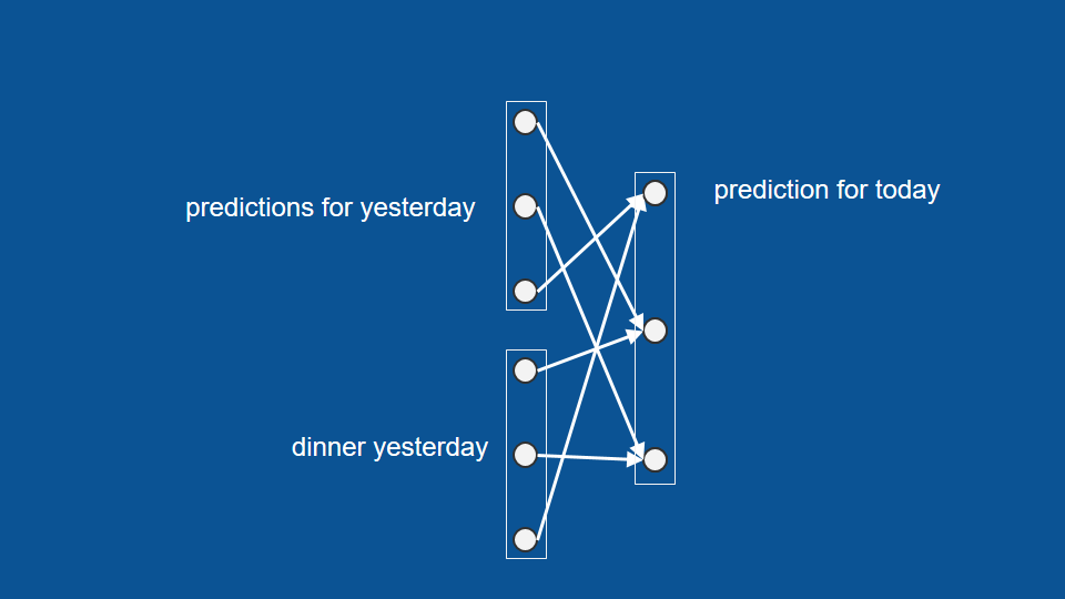
今天的預測結果如何在明天被重新利用,成為明天的「昨日預測」:
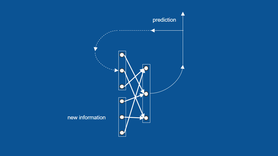
換一個寫童書的例子。這本童書裡只有三種句子:
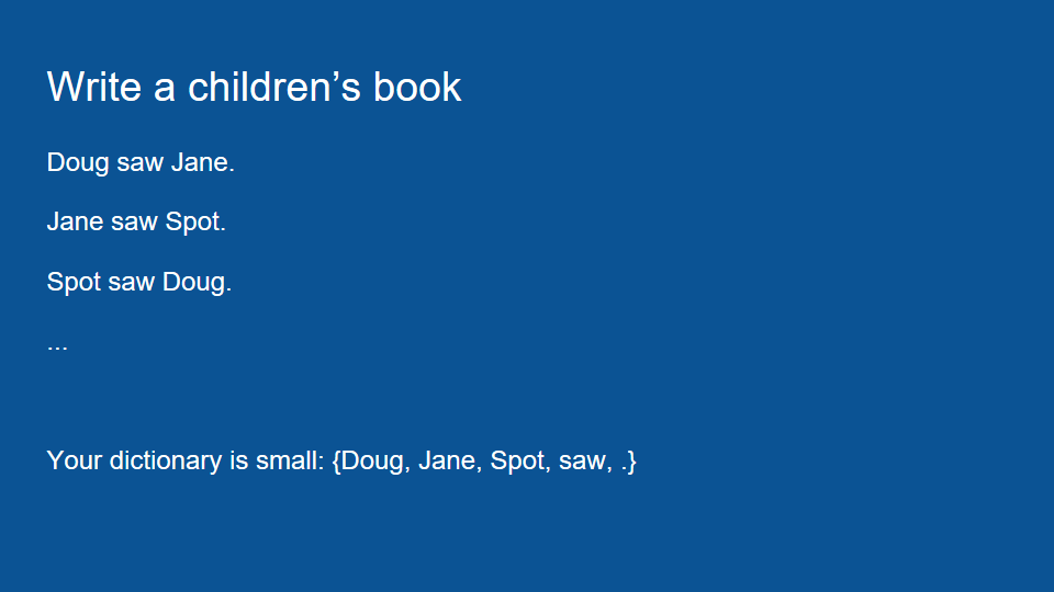
這本童書的字彙量很小,只有「Doug」、「Jane」、「Spot」、「saw」以及句號。
經過一定的訓練後,我們應該能從模型中看出一些特定的規律: 像是在「Jane、Doug、Spot」之後,模型預測「saw」和句點的機率應該會大幅提升,因為這兩個單字都會跟著特定名字出現。
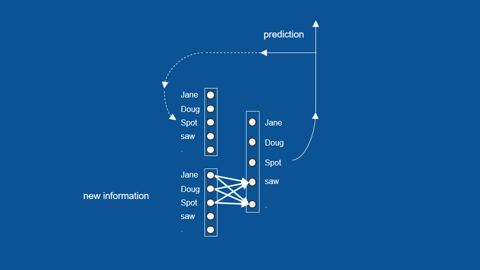
同樣地,如果我們前一次預測了名字,那這些預測也會增加接下來預測「saw」或句號的機率
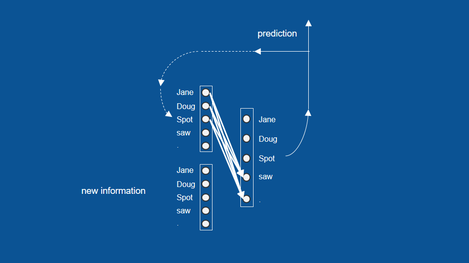
如果我們看到「saw」或句號,也能想像模型接下來會傾向於預測「Jane、Doug、Spot」等名字。

這個例子裡的神經網路會出現一些錯誤,像是得出「道格看見道格(句號)」等句子,因為每當「看見」出現在模型裡,後面接著名字的機率就會大幅提升。
這是因為我們的模型有著很短期的記憶,只會參考前一步的結果,為了解決這個問題,我們需要在模型中加入更多內容: 記憶/遺忘路徑.
透過Logistic函數(sigmoid),建立一個回憶或遺忘特定資訊的gate(即圖中的「圈叉」符號),並將結果加回下次的預測當中 (即圖中的「圈加」符號) 。
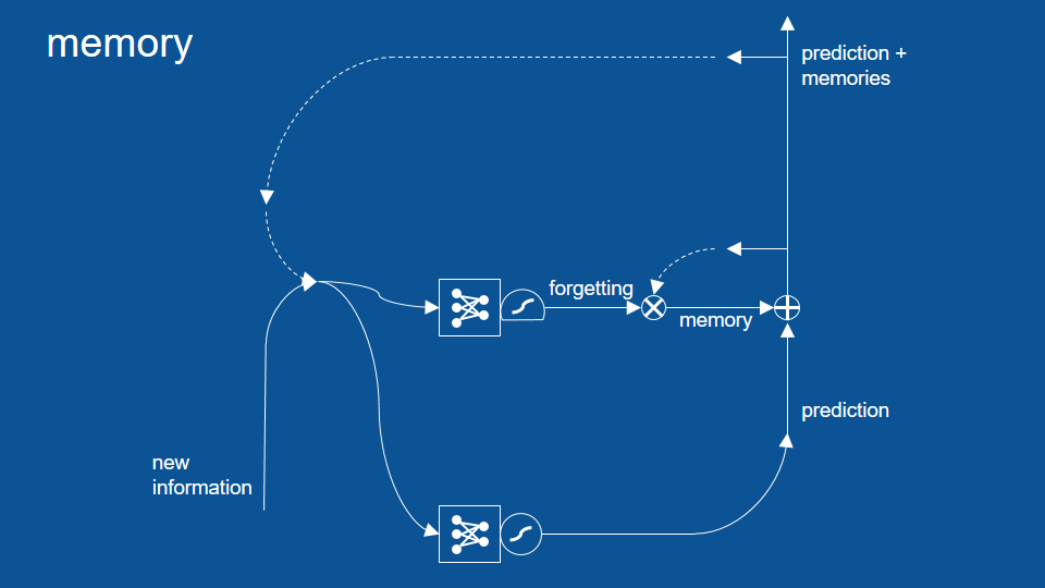
擠壓函數(squashing function,又譯作 S 函數)的處理,對於神經網路這種重複運算相同數值的流程非常有用。
藉由S函數確保數值介於 1 和 -1 之間,即使我們將數值相乘無數次,也不用擔心它會在循環中無限增大。這是一種負回饋(negative feedback)或衰減回饋(attenuating feedback)的例子。
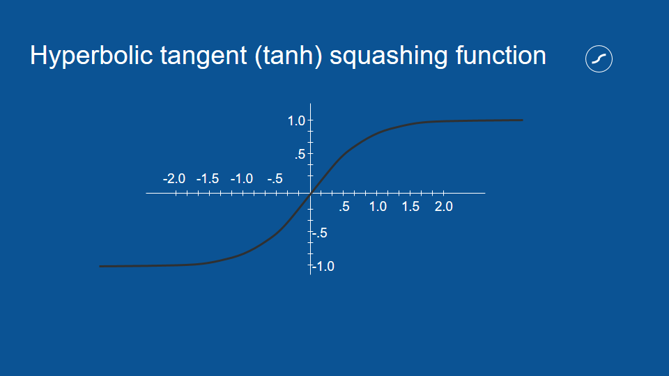
為了得到一組介於 0 和 1 之間的數值,所以這裡又有另一種壓縮函數。這個函數的符號是一個帶有平底的圓形,它被稱作邏輯函數(logistic function)。
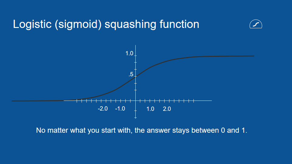
In the conventional feed-forward neural networks, all test cases are considered to be independent.
An RNN is a type of neural network that has an internal loop : it processes sequences by iterating through the sequence elements and maintaining a state containing information relative to what it has seen so far. Therefore, the dependency on time is achieved.
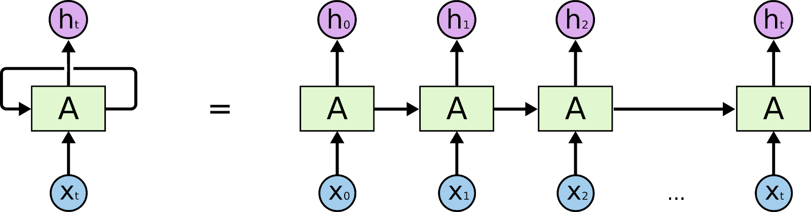
Here is the pseudo code:
state_t = 0
for input_t in input_sequence:
output_t = activation( dot(W, input_t) + dot(U, state_t) + b)
state_t = output_t
For example: x has the following sequence data.
x = [1,2,3,4,5,6,7,8,9,10]y is its prediction :
- for step=1, x and y contain:
x y 1 2 2 3 3 4 4 5 .. 9 10
x y 1,2,3 4 2,3,4 5 3,4,5 6 4,5,6 7 ... 7,8,9 10To make these notions of loop and state clear,
The RNN takes as input a sequence of vectors, which you’ll encode as a 2D tensor of size (timesteps, input_features) . It loops over timesteps, and at each timestep, it considers its current state at t and the input at t (of shape (input_features,) , and combines them to obtain the output at t . RNN usually wants to predict a vector at some time steps.Numpy implementation of a simple RNN
import numpy as np
timesteps = 100
input_features = 32
output_features = 64
inputs = np.random.random((timesteps, input_features))
state_t = np.zeros((output_features,))
W = np.random.random((output_features, input_features))
U = np.random.random((output_features, output_features))
b = np.random.random((output_features,))
successive_outputs = []
for input_t in inputs:
output_t = np.tanh(np.dot(W, input_t) + np.dot(U, state_t) + b)
successive_outputs.append(output_t)
state_t = output_t
final_output_sequence = np.concatenate(successive_outputs, axis=0)
6.2.1 A recurrent layer in Keras
Recurrent Neural Network models can be easily built in a Keras API.
keras.layers.SimpleRNN(units, activation='tanh',
use_bias=True, kernel_initializer='glorot_uniform',
recurrent_initializer='orthogonal', bias_initializer='zeros',
kernel_regularizer=None, recurrent_regularizer=None,
bias_regularizer=None, activity_regularizer=None,
kernel_constraint=None, recurrent_constraint=None,
bias_constraint=None, dropout=0.0, recurrent_dropout=0.0,
return_sequences=False, return_state=False,
go_backwards=False, stateful=False, unroll=False)
- return_sequences Decide either the full sequences of successive outputs for each timestep (a 3D tensor of shape (batch_size, timesteps, output_features) ) or only the last output for each input sequence (a 2D tensor of shape (batch_size, output_features) ) is returned. That is, the output shape is decided by this parameter. You can use model.summary() to check the shape of the output.
model = Sequential()
model.add(Embedding(10000, 32))
- model.add(SimpleRNN(32))
Layer (type) Output Shape Param #
================================================================
embedding_22 (Embedding)(None, None, 32) 320000
________________________________________________________________
simplernn_10 (SimpleRNN)(None, 32) 2080
================================================================
________________________________________________________________
Layer (type) Output Shape Param #
================================================================
embedding_23 (Embedding)(None, None, 32) 320000
________________________________________________________________
simplernn_11 (SimpleRNN)(None, None, 32) 2080
================================================================
- Preparing the IMDB data
from keras.datasets import imdb
from keras.preprocessing import sequence
from keras.layers import Embedding, Dense, SimpleRNN
# Number of words to consider as features
max_features = 10000
# Cuts off reviews ( < max_features most common words)
maxlen = 500
batch_size = 32
print('Loading data...')
(input_train, y_train), (input_test, y_test) = imdb.load_data(num_words=max_features)
print(len(input_train), 'train sequences')
print(len(input_test), 'test sequences')
print('Pad sequences (samples x time)')
input_train = sequence.pad_sequences(input_train, maxlen=maxlen)
input_test = sequence.pad_sequences(input_test, maxlen=maxlen)
print('input_train shape:', input_train.shape)
print('input_test shape:', input_test.shape)
from keras.layers import Dense
model = Sequential()
model.add(Embedding(max_features, 32))
model.add(SimpleRNN(32))
model.add(Dense(1, activation='sigmoid'))
model.compile(optimizer='rmsprop', loss='binary_crossentropy', metrics=['acc'])
history = model.fit(input_train, y_train,
epochs=10,
batch_size=128,
validation_split=0.2)
import matplotlib.pyplot as plt
acc = history.history['acc']
val_acc = history.history['val_acc']
loss = history.history['loss']
val_loss = history.history['val_loss']
epochs = range(1, len(acc) + 1)
plt.plot(epochs, acc, 'bo', label='Training acc')
plt.plot(epochs, val_acc, 'b', label='Validation acc')
plt.title('Training and validation accuracy')
plt.legend()
plt.figure()
plt.plot(epochs, loss, 'bo', label='Training loss')
plt.plot(epochs, val_loss, 'b', label='Validation loss')
plt.title('Training and validation loss')
plt.legend()
plt.show()
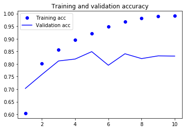
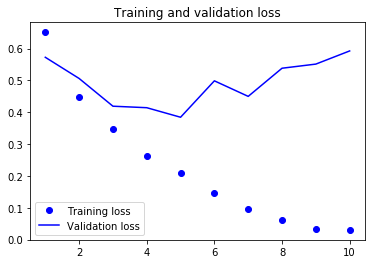
Unfortunately, this small recurrent network doesn’t perform well, SimpleRNN isn’t good at processing long sequences, such as text
6.2.2 Understanding the LSTM and GRU layers
SimpleRNN is generally too simplistic to be of real use.
Sometimes, we only need to look at recent information to perform the present task. In such cases, where the gap between the relevant information and the place that it’s needed is small, RNNs can learn to use the past information.
But there are also cases where we need more context. Unfortunately, as that gap grows, RNNs become unable to learn to connect the information.
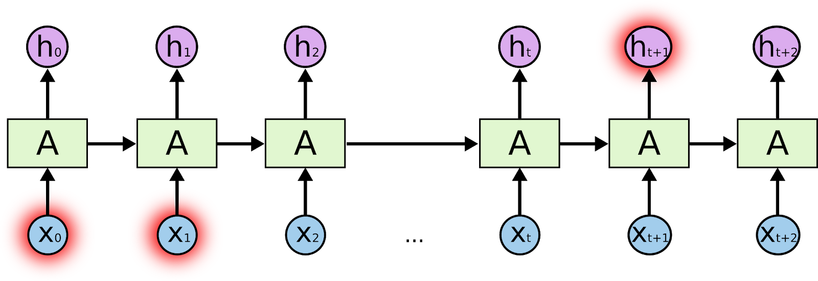
There are two other RNN layers abailable in keras: LSTM(Long Short-Term Memory) and GRU .
LSTMs have been observed as the most effective solution for Sequence prediction problems . It is a variant of the SimpleRNN layer: it makes small modifications to the previous information by multiplications and additions.
LSTMs are explicitly designed to avoid the long-term dependency problem.
All recurrent neural networks have the form of a chain of repeating modules of neural network.
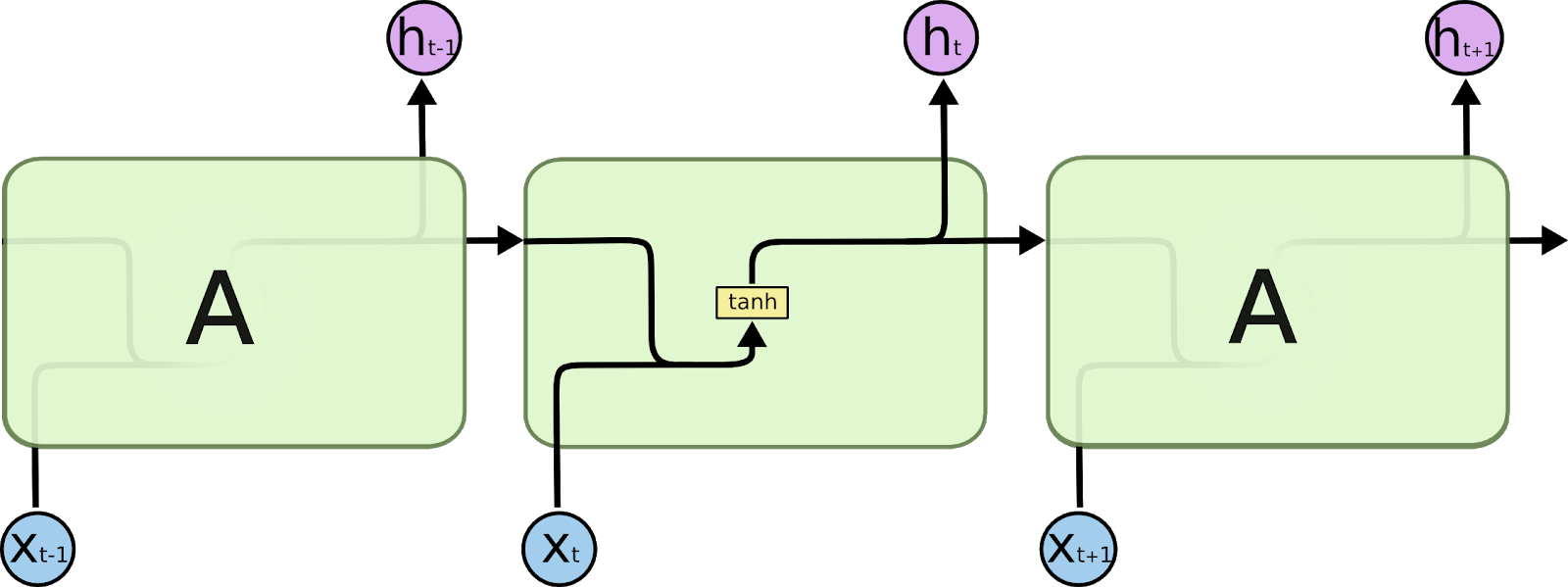
LSTMs also have this chain like structure, but the repeating module has 4, interacting in a very special way.
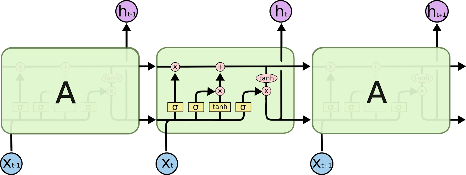
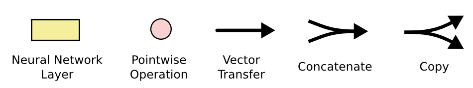
The Core Idea Behind LSTMs:
A typical LSTM network is comprised of different memory blocks called cells.
There are 2 states that are being transferred to the next cell; the cell state and the hidden state.
Cells use 3 major mechanisms, called gates, to remember and operate the memory:
- Forget Gate This controls when the current context/subject is ended. A forget gate is responsible for removing information from the cell state. The information that is no longer required for the LSTM to understand things or the information that is of less importance is removed via multiplication of a filter.
- h(t-1) The hidden state from the previous cell or the output of the previous cell.
- x(t) The input at that particular time step.
- Input Gate
- Output Gate
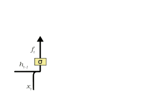 This gate takes in two inputs:
 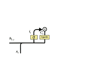 The input gate is responsible for the addition of information(important and is not redundant) to the cell state.
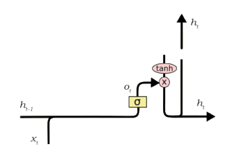 This job of selecting useful information from the current cell state and showing it out as an output is done via the output gate.
 6.2.3 A concrete LSTM example in Keras
keras.layers.LSTM(units, activation='tanh', recurrent_activation='sigmoid',
use_bias=True, kernel_initializer='glorot_uniform', recurrent_initializer='orthogonal',
bias_initializer='zeros', unit_forget_bias=True, kernel_regularizer=None,
recurrent_regularizer=None, bias_regularizer=None, activity_regularizer=None,
kernel_constraint=None, recurrent_constraint=None, bias_constraint=None, dropout=0.0,
recurrent_dropout=0.0, implementation=2, return_sequences=False, return_state=False,
go_backwards=False, stateful=False, unroll=False)
Text generation using LSTMs:
Use LSTM to solve a sequence prediction task.
- mporting dependencies
# Importing dependencies numpy and keras import numpy from keras.models import Sequential from keras.layers import Dense from keras.layers import Dropout from keras.layers import LSTM from keras.utils import np_utils
import os dir_name = '/content/gdrive/My Drive/Colab/Datasets/Shakespeare' # load text fname = "macbeth.txt" text = (open(os.path.join(dir_name, fname)).read()).lower() # mapping characters with integers unique_chars = sorted(list(set(text))) char_to_int = {} int_to_char = {} for i, c in enumerate (unique_chars): char_to_int.update({c: i}) int_to_char.update({i: c})
The trained data is prepared in a format such that if we want the LSTM to predict the ‘O’ in ‘HELLO’ we would feed in [‘H’, ‘E‘ , ‘L ‘ , ‘L‘ ] as the input and [‘O’] as the expected output. In this case,# preparing input and output dataset X = [] Y = [] for i in range(0, len(text) - 50, 1): sequence = text[i:i + 50] label =text[i + 50] X.append([char_to_int[char] for char in sequence]) Y.append(char_to_int[label])
- the length of the sequence is set to 50
- the encodings of the first 50 characters starting for each character is saved in X X is a list of encoded sequence having length 50. Y is a list of character which is the 51-th character for X.
- the expected output i.e. the 51-th character in Y.
A LSTM network expects the input to be in the form :# reshaping, normalizing and one hot encoding X_modified = numpy.reshape(X, (len(X), 50, 1)) X_modified = X_modified / float(len(unique_chars)) Y_modified = np_utils.to_categorical(Y)
[samples, time steps, features]
- samples is the number of data points we have
- time steps is the number of time-dependent steps that are there in a single data point
- features refers to the number of variables we have for the corresponding true value in Y.
A sequential model which is a linear stack of layers :# defining the LSTM model model = Sequential() model.add(LSTM(300, input_shape=(X_modified.shape[1], X_modified.shape[2]), return_sequences=True)) model.add(Dropout(0.2)) model.add(LSTM(300)) model.add(Dropout(0.2)) model.add(Dense(Y_modified.shape[1], activation='softmax')) model.compile(loss='categorical_crossentropy', optimizer='adam')
- A LSTM layer with 300 memory units
- A dropout layer is applied after each LSTM layer to avoid overfitting of the model.
- A fully connected layer with a ‘softmax’ activation and neurons equal to the number of unique characters
Jerry's comment:# fitting the model model.fit(X_modified, Y_modified, epochs=1, batch_size=30) # save the model model.save(f"/content/gdrive/My Drive/Colab/Models/shakespeare-Macbeth.model.hdf5") # picking a random seed start_index = numpy.random.randint(0, len(X)-1) new_string = X[start_index] # generating characters for i in range(50): #print(new_string) x = numpy.reshape(new_string, (1, len(new_string), 1)) x = x / float(len(unique_chars)) #predicting on new data pred_index = numpy.argmax(model.predict(x, verbose=0)) char_out = int_to_char[pred_index] seq_in = [int_to_char[value] for value in new_string] print( char_out, 'is for: ', int_to_char[Y[start_index + i]], seq_in) new_string.append(pred_index) new_string = new_string[1:len(new_string)]
I believe this is a good example to illustrate the usage of the Keras API but a bad usage case.
According to the result, the train set is not designed well to predict a character after a sequence of 50 characters.
It may be a better case to predict a word in a sentence.
Let's try a better usage case.
Set up a model using an LSTM layer and train it on the IMDB data:
- Preparing the IMDB data
from keras.datasets import imdb
from keras.preprocessing import sequence
from keras.layers import Embedding, Dense, SimpleRNN
# Number of words to consider as features
max_features = 10000
# Cuts off reviews ( < max_features most common words)
maxlen = 500
batch_size = 32
print('Loading data...')
(input_train, y_train), (input_test, y_test) = imdb.load_data(num_words=max_features)
print('Pad sequences (samples x time)')
input_train = sequence.pad_sequences(input_train, maxlen=maxlen)
input_test = sequence.pad_sequences(input_test, maxlen=maxlen)
print('input_train shape:', input_train.shape)
print('input_test shape:', input_test.shape)
from keras.layers import LSTM
model = Sequential()
model.add(Embedding(max_features, 32))
model.add(LSTM(32))
model.add(Dense(1, activation='sigmoid'))
model.compile(optimizer='rmsprop',
loss='binary_crossentropy',
metrics=['acc'])
history = model.fit(input_train, y_train,
epochs=10,
batch_size=128,
validation_split=0.2)
import matplotlib.pyplot as plt

acc = history.history['acc']
val_acc = history.history['val_acc']
loss = history.history['loss']
val_loss = history.history['val_loss']
epochs = range(1, len(acc) + 1)
plt.plot(epochs, acc, 'bo', label='Training acc')
plt.plot(epochs, val_acc, 'b', label='Validation acc')
plt.title('Training and validation accuracy')
plt.legend()
plt.figure()
plt.plot(epochs, loss, 'bo', label='Training loss')
plt.plot(epochs, val_loss, 'b', label='Validation loss')
plt.title('Training and validation loss')
plt.legend()
plt.show()
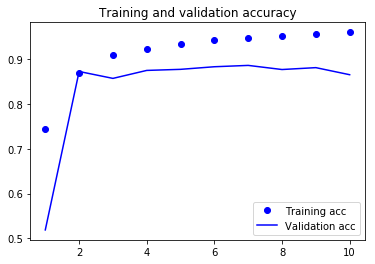
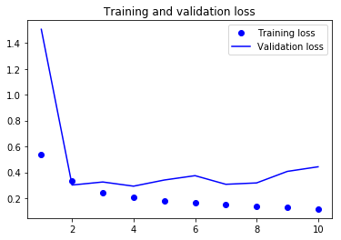 The result of LSTM is better than the RNN.
 6.3 Advanced use of recurrent neural networks
We’ll demonstrate using a temperature-forecasting problem:
A timeseries of data points coming from sensors installed on the roof of a building to predict what the temperature will be 24 hours after the last data point.
- temperature
- air pressure
- humidity
- ...
6.3.1 A temperature-forecasting problem
You’ll play with a weather timeseries dataset recorded, 14 different quantities (such air temperature, atmospheric pressure, humidity, wind direction, and so on) were recorded every 10 minutes, over several years.
- Download and uncompress the data
cd ~/Downloads
mkdir jena_climate
cd jena_climate
wget https://s3.amazonaws.com/keras-datasets/jena_climate_2009_2016.csv.zip
unzip jena_climate_2009_2016.csv.zip
import os

dir_name = '/content/gdrive/My Drive/Colab/Datasets'
fname = os.path.join(data_dir, 'jena_climate_2009_2016.csv')
f = open(fname)
data = f.read()
f.close()
lines = data.split('\n')
# 1st line is the header
header = lines[0].split(',')
# data following the header
lines = lines[1:]
print(header)
print(len(lines))
  "Date Time","p (mbar)","T (degC)","Tpot (K)","Tdew (degC)","rh (%)","VPmax (mbar)","VPact (mbar)","VPdef (mbar)","sh (g/kg)","H2OC (mmol/mol)","rho (g/m**3)","wv (m/s)","max. wv (m/s)","wd (deg)"
  01.01.2009 00:10:00,996.52,-8.02,265.40,-8.90,93.30,3.33,3.11,0.22,1.94,3.12,1307.75,1.03,1.75,152.30
import numpy as np

float_data = np.zeros((len(lines), len(header) - 1))
for i, line in enumerate(lines):
    # skip the "Date Time" field
    values = [float(x) for x in line.split(',')[1:]]
    float_data[i, :] = values
from matplotlib import pyplot as plt

temp = float_data[:, 1]
plt.plot(range(len(temp)), temp)
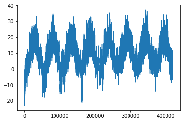 The first 10 days of temperature data:
plt.plot(range(1440), temp[:1440])
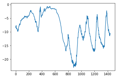 The year-scale periodicity of the data can be easily seen. Is this timeseries predictable at a daily scale?
 6.3.2 Preparing the data
The exact formulation of the problem:
- Observations will go back 5 days. A timestep is 10 minutes so that 720 timesteps are for lookback. ( 5 * 24 * 60 / 10 = 720 )
- Observations will be sampled at one data point per hour Observation will happen every 6 steps.
- Prediction will be 24 hours in the future Prediction is delayed with 144 steps.
- Normalizing the data
Each timeseries in the data is on a different scale, you’ll normalize each timeseries independently so that they all take small values on a similar scale. The first 200,000 timesteps are as training data
mean = float_data[:200000].mean(axis=0) float_data -= mean std = float_data[:200000].std(axis=0) float_data /= std - Define a generator yielding timeseries samples and their targets
def generator(data, lookback, delay, min_index, max_index,
    shuffle=False, batch_size=128, step=6):
    if max_index is None:
        max_index = len(data) - delay - 1
    i = min_index + lookback
    while 1:
        if shuffle:
            rows = np.random.randint(min_index + lookback, max_index, size=batch_size)
        else:
            if i + batch_size >= max_index:
                i = min_index + lookback
            rows = np.arange(i, min(i + batch_size, max_index))
            i += len(rows) # reset i
        # indices of samples (row) is decided
        samples = np.zeros((len(rows),
            lookback // step,
            data.shape[-1]))
        targets = np.zeros((len(rows),))
        for j, row in enumerate(rows):
            indices = range(rows[j] - lookback, rows[j], step)
            # related input sequence for a timestamp
            samples[j] = data[indices]
            # prediction happens at the timestamp + delay
            targets[j] = data[rows[j] + delay][1] # temp = float_data[:, 1]
        yield samples, targets
- data — The original array of floating-point data which you normalized in the previous step
- lookback — How many timesteps back the input data should go.
- delay — How many timesteps in the future the target should be.
- min_index and max_index — Indices the range in the data array to draw from for this generator. This is useful for keeping a segment of the data for validation and another for testing.
- shuffle — Whether to shuffle the samples or draw them in chronological order.
- batch_size — The number of samples per batch.
- step — The period, in timesteps, at which you sample data. You’ll set it to 6 in order to draw one data point every hour.
We'll initiate 3 generators: the training generator looks at the first 200,000 timesteps, the validation generator looks at the following 100,000, and the test generator looks at the remainder.
lookback = 1440
step = 6
delay = 144
batch_size = 128

train_gen = generator(float_data,
    lookback=lookback,
    delay=delay,
    min_index=0,
    max_index=200000,
    shuffle=True,
    step=step,
    batch_size=batch_size)
val_gen = generator(float_data,
    lookback=lookback,
    delay=delay,
    min_index=200001,
    max_index=300000,
    step=step,
    batch_size=batch_size)
test_gen = generator(float_data,
    lookback=lookback,
    delay=delay,
    min_index=300001,
    max_index=None,
    step=step,
    batch_size=batch_size)

# How many steps to draw from val_gen
# in order to see the entire validation set
val_steps = (300000 - 200001 - lookback)

# How many steps to draw from test_gen
# in order to see the entire test set
test_steps = (len(float_data) - 300001 - lookback)
6.3.3 A common-sense, non-machine-learning baseline
A common-sense approach is to always predict that the temperature 24 hours from now will be equal to the temperature right now.6.3.4 A basic machine-learning approach
Training and evaluating a densely connected model:
from keras.models import Sequential
from keras import layers
from keras.optimizers import RMSprop

model = Sequential()
model.add(layers.Flatten(input_shape=(lookback // step, float_data.shape[-1])))
model.add(layers.Dense(32, activation='relu'))
model.add(layers.Dense(1))
model.compile(optimizer=RMSprop(), loss='mae')
history = model.fit_generator(train_gen,
  steps_per_epoch=500,
  epochs=20,
  validation_data=val_gen,
  validation_steps=val_steps)
import matplotlib.pyplot as plt

loss = history.history['loss']
val_loss = history.history['val_loss']
epochs = range(1, len(loss) + 1)
plt.figure()
plt.plot(epochs, loss, 'bo', label='Training loss')
plt.plot(epochs, val_loss, 'b', label='Validation loss')
plt.title('Training and validation loss')
plt.legend()
plt.show()
6.3.5 A first recurrent baseline
Gated recurrent units (GRUs) are a gating mechanism in recurrent neural networks, introduced in 2014 by Kyunghyun Cho et al. The GRU is like a long short-term memory (LSTM) with forget gate but has fewer parameters than LSTM, as it lacks an output gate. Training and evaluating a GRU-based model:
from keras.models import Sequential
from keras import layers
from keras.optimizers import RMSprop

model = Sequential()
model.add(layers.GRU(32, input_shape=(None, float_data.shape[-1])))
model.add(layers.Dense(1))
model.compile(optimizer=RMSprop(), loss='mae')
history = model.fit_generator(train_gen,
  steps_per_epoch=500,
  epochs=20,
  validation_data=val_gen,
  validation_steps=val_steps)
6.3.6 Using recurrent dropout to fight overfitting
Every recurrent layer in Keras has two dropout-related arguments:- dropout a float specifying the dropout rate for input units of the layer
- recurrent_dropout specifying the dropout rate of the recurrent units.
from keras.models import Sequential
from keras import layers
from keras.optimizers import RMSprop

model = Sequential()
model.add(layers.GRU(32,
  dropout=0.2, recurrent_dropout=0.2,
input_shape=(None, float_data.shape[-1])))
model.add(layers.Dense(1))
model.compile(optimizer=RMSprop(), loss='mae')
history = model.fit_generator(train_gen,
  steps_per_epoch=500,
  epochs=40,
  validation_data=val_gen,
  validation_steps=val_steps)
6.3.7 Stacking recurrent layers
6.3.8 Using bidirectional RNNs
6.3.9 Going even further
6.4 Sequence processing with convnets
Time can be treated as a spatial dimension, like the height or width of a 2D image. Such 1D convnets can be competitive with RNNs on certain sequence-processing problems. Recently, 1D convnets, typically used with dilated kernels, have been used with great success for audio generation and machine translation. In addition to these specific successes, it has long been known that small 1D convnets can offer a fast alternative to RNN s for simple tasks such as text classification and timeseries forecasting.6.4.1 Understanding 1D convolution for sequence data
With the same way, you can use 1D convolutions(1D kernel), extracting local 1D patches (subsequences) from sequences,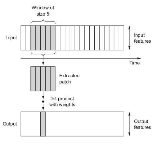
6.4.2 1D pooling for sequence data
Just as with 2D convnets, this is used for reducing the length of 1D inputs (subsampling).6.4.3 Implementing a 1D convnet
In Keras, you use a 1D convnet via the Conv1D layer.
keras.layers.Conv1D(filters, kernel_size,
    strides=1, padding='valid', data_format='channels_last',
    dilation_rate=1, activation=None, use_bias=True,
    kernel_initializer='glorot_uniform', bias_initializer='zeros',
    kernel_regularizer=None, bias_regularizer=None,
    activity_regularizer=None, kernel_constraint=None,
    bias_constraint=None)
- channels_last (batch, steps, channels)
- channels_first (batch, channels, steps)
- Preparing the IMDB data
from keras.datasets import imdb
from keras.preprocessing import sequence

max_features = 10000
max_len = 500
print('Loading data...')
(x_train, y_train), (x_test, y_test) = imdb.load_data(num_words=max_features)
print(len(x_train), 'train sequences')
print(len(x_test), 'test sequences')
print('Pad sequences (samples x time)')
x_train = sequence.pad_sequences(x_train, maxlen=max_len)
x_test = sequence.pad_sequences(x_test, maxlen=max_len)
print('x_train shape:', x_train.shape)
print('x_test shape:', x_test.shape)
25000 train sequences
25000 test sequences
Pad sequences (samples x time)
x_train shape: (25000, 500)
x_test shape: (25000, 500)
from keras.models import Sequential
from keras import layers
from keras.optimizers import RMSprop

model = Sequential()
model.add(layers.Embedding(max_features, 128, input_length=max_len))
model.add(layers.Conv1D(32, 7, activation='relu'))
model.add(layers.MaxPooling1D(5))
model.add(layers.Conv1D(32, 7, activation='relu'))
model.add(layers.GlobalMaxPooling1D())
model.add(layers.Dense(1))
model.summary()

model.compile(optimizer=RMSprop(lr=1e-4),
  loss='binary_crossentropy',
  metrics=['acc'])

history = model.fit(x_train, y_train,
  epochs=10,
  batch_size=128,
  validation_split=0.2)
Model: "sequential_1"
_________________________________________________________________
Layer (type)                 Output Shape              Param #
=================================================================
embedding_1 (Embedding)      (None, 500, 128)          1280000
_________________________________________________________________
conv1d_1 (Conv1D)            (None, 494, 32)           28704
_________________________________________________________________
max_pooling1d_1 (MaxPooling1 (None, 98, 32)            0
_________________________________________________________________
conv1d_2 (Conv1D)            (None, 92, 32)            7200
_________________________________________________________________
global_max_pooling1d_1 (Glob (None, 32)                0
_________________________________________________________________
dense_1 (Dense)              (None, 1)                 33
=================================================================
Total params: 1,315,937
Trainable params: 1,315,937
Non-trainable params: 0

20000/20000 [==============================] - 93s 5ms/step - loss: 0.2226 - acc: 0.7989 - val_loss: 0.4497 - val_acc: 0.7452
import matplotlib.pyplot as plt

loss = history.history['loss']
val_loss = history.history['val_loss']
epochs = range(1, len(loss) + 1)
plt.figure()
plt.plot(epochs, loss, 'bo', label='Training loss')
plt.plot(epochs, val_loss, 'b', label='Validation loss')
plt.title('Training and validation loss')
plt.legend()
plt.show()
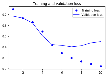
6.4.4 Combining CNNs and RNNs to process long sequences
7 Advanced deep-learning best practices
7.1 Going beyond the Sequential model: the Keras functional API
Some Input networks require several independent inputs, others require multiple outputs, and some networks have internal branching between layers that makes them look like graphs of layers rather than linear stacks of layers. Imagine a deep-learning model trying to predict the most likely market price of a second-hand piece of clothing, using the following inputs: user-provided metadata(such as the item’s brand, age, and so on), a user-provided text description, and a picture of the item. A better way is to jointly learn a more accurate model of the data by using a model that can see all available input modalities simultaneously: a model with three input branches.Metadata ----------> Dense Module ---+---------+
| Merging |
Text description --> RNN Module -----+ +--- Price prediction
| module |
Picture -----------> Convnet module--+---------+
There’s another far more general and flexible way to use Keras: the functional API . 7.1.1 Introduction to the functional API
In the functional API , you directly manipulate tensors, and you use layers as functions that take tensors and return tensors:
from keras import Input, layers

# An input tensor
input_tensor = Input(shape=(32,))
# A layer is initialized as a function
dense = layers.Dense(32, activation='relu')
# A layer function is called to operate on a tensor, and it returns a tensor
output_tensor = dense(input_tensor)
from keras.models import Model
from keras import layers
from keras import Input

input_tensor = Input(shape=(64,))
x = layers.Dense(32, activation='relu')(input_tensor)
x = layers.Dense(32, activation='relu')(x)
output_tensor = layers.Dense(10, activation='softmax')(x)
model = Model(input_tensor, output_tensor)
model.summary()
Model: "model_1"
_________________________________________________________________
Layer (type)                 Output Shape              Param #
=================================================================
input_1 (InputLayer)         (None, 64)                0
_________________________________________________________________
dense_2 (Dense)              (None, 32)                2080
_________________________________________________________________
dense_3 (Dense)              (None, 32)                1056
_________________________________________________________________
dense_4 (Dense)              (None, 10)                330
=================================================================
Total params: 3,466
Trainable params: 3,466
Non-trainable params: 0
Behind the scenes, Keras retrieves every layer involved in going from input_tensor to output_tensor , bringing them together into a graph-like data structure — a Model . The output_tensor was obtained by repeatedly transforming input_tensor .
7.1.2 Multi-input models
The functional API can be used to build models that have multiple inputs. This is usually done via a Keras merge operation such as keras.layers.add , keras.layers.concatenate , and so on. A typical question-answering model: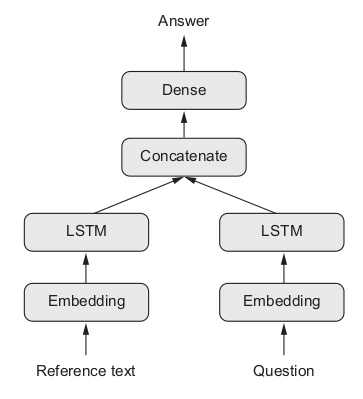
An example of how you can build such a model with the functional API . - Initial setup
from keras.models import Model
from keras import layers
from keras import Input

text_vocabulary_size = 10000
question_vocabulary_size = 10000
answer_vocabulary_size = 500
from keras.models import Model
from keras import layers
from keras import Input
text_vocabulary_size = 10000
question_vocabulary_size = 10000
answer_vocabulary_size = 500
text_input = Input(shape=(None,), dtype='int32', name='text')
embedded_text = layers.Embedding(64, text_vocabulary_size)(text_input)
encoded_text = layers.LSTM(32)(embedded_text)
question_input = Input(shape=(None,), dtype='int32', name='question')
embedded_question = layers.Embedding(32, question_vocabulary_size)(question_input)
encoded_question = layers.LSTM(16)(embedded_question)
concatenated = layers.concatenate([encoded_text, encoded_question], axis=-1)
answer = layers.Dense(answer_vocabulary_size,
  activation='softmax')(concatenated)
model = Model([text_input, question_input], answer)
model.compile(optimizer='rmsprop',
  loss='categorical_crossentropy',
  metrics=['acc'])
import numpy as np

# Generates dummy Numpy data
num_samples = 1000
max_length = 100
text = np.random.randint(1, text_vocabulary_size, size=(num_samples, max_length))
question = np.random.randint(1, question_vocabulary_size, size=(num_samples, max_length))
# Answers are one-hot encoded, not integers
answers = np.random.randint(0, 1, size=(num_samples, answer_vocabulary_size))
model.fit([text, question], answers, epochs=10, batch_size=128)
7.1.4 Directed acyclic graphs of layers
7.1.5 Layer weight sharing
7.1.6 Models as layers
7.2 Inspecting and monitoring deep-learning models using Keras callbacks and TensorBoard
There are ways to gain greater access to and control over what goes on inside your model during training.7.2.1 Using callbacks to act on a model during training
A better way to stop training is when you measure that the validation loss in no longer improving. This can be achieved using a Keras callback. A callback is an object (a class instance implementing specific methods) that is passed to the model in the call to fit and that is called by the model at various points during training. Callbacks have access to all the available data about the state of the model and its performance, and it can take action:- Model checkpointing Saving the current weights of the model at different points during training.
- Early stopping Interrupting training when the validation loss is no longer improving (and of course, saving the best model obtained during training).
- Dynamically adjusting the value of certain parameters during training Such as the learning rate of the optimizer.
- Logging training and validation metrics during training, or visualizing the representations learned by the model as they’re updated The Keras progress bar that you’re familiar with is a callback!
- keras.callbacks.callbacks.BaseLogger(stateful_metrics=None) Callback that accumulates epoch averages of metrics.
- keras.callbacks.callbacks.TerminateOnNaN() Callback that terminates training when a NaN loss is encountered.
- keras.callbacks.callbacks.ProgbarLogger(count_mode='samples', stateful_metrics=None) Callback that prints metrics to stdout.
- keras.callbacks.callbacks.History() Callback that records events into a History object. This callback is automatically applied to every Keras model. The History object gets returned by the fit method of models.
- keras.callbacks.callbacks.ModelCheckpoint(filepath, monitor='val_loss', verbose=0, save_best_only=False, save_weights_only=False, mode='auto', period=1) Save the model after every epoch. filepath can contain named formatting options, which will be filled with the values of epoch and keys in logs (passed in on_epoch_end). For example: if filepath is weights.{epoch:02d}-{val_loss:.2f}.hdf5, then the model checkpoints will be saved with the epoch number and the validation loss in the filename.
- keras.callbacks.callbacks.EarlyStopping(monitor='val_loss', min_delta=0, patience=0, verbose=0, mode='auto', baseline=None, restore_best_weights=False) Stop training when a monitored quantity has stopped improving.
- keras.callbacks.callbacks.RemoteMonitor(root='http://localhost:9000', path='/publish/epoch/end/', field='data', headers=None, send_as_json=False) Callback used to stream events to a server.
- keras.callbacks.callbacks.LearningRateScheduler(schedule, verbose=0) Learning rate scheduler.
- keras.callbacks.callbacks.ReduceLROnPlateau(monitor='val_loss', factor=0.1, patience=10, verbose=0, mode='auto', min_delta=0.0001, cooldown=0, min_lr=0) Reduce learning rate when a metric has stopped improving.
- keras.callbacks.callbacks.CSVLogger(filename, separator=',', append=False) Callback that streams epoch results to a csv file.
- keras.callbacks.callbacks.LambdaCallback(on_epoch_begin=None, on_epoch_end=None, on_batch_begin=None, on_batch_end=None, on_train_begin=None, on_train_end=None) Callback for creating simple, custom callbacks on-the-fly.
- keras.callbacks.tensorboard_v1.TensorBoard(log_dir='./logs', histogram_freq=0, batch_size=32, write_graph=True, write_grads=False, write_images=False, embeddings_freq=0, embeddings_layer_names=None, embeddings_metadata=None, embeddings_data=None, update_freq='epoch') TensorBoard is a visualization tool provided with TensorFlow. This callback writes a log for TensorBoard, which allows you to visualize dynamic graphs of your training and test metrics, as well as activation histograms for the different layers in your model. If you have installed TensorFlow with pip, you should be able to launch TensorBoard from the command line:
tensorboard --logdir=/full_path_to_your_logs
import keras

callbacks_list = [
  keras.callbacks.EarlyStopping(
    monitor='acc', # Monitors the model’s validation accuracy
    patience=1,), # Interrupt training when accuracy has stopped improving for more than one epoch
  keras.callbacks.ModelCheckpoint(
    filepath='my_model.h5',
    monitor='val_loss', # Monitors the model’s validation loss
    save_best_only=True,)
]

model.compile(optimizer='rmsprop',
  loss='binary_crossentropy',
  metrics=['acc'])

model.fit(x, y,
  epochs=10,
  batch_size=32,
  callbacks=callbacks_list,
  validation_data=(x_val, y_val))
callbacks_list = [
keras.callbacks.ReduceLROnPlateau(
monitor='val_loss',
factor=0.1, # Divides the learning rate by 10 when triggered
patience=10,), # Interrupt training when validation loss has stopped improving for more than 10 epoch
]
model.fit(x, y,
epochs=10,
batch_size=32,
callbacks=callbacks_list,
validation_data=(x_val, y_val))
- on_epoch_begin Called at the start of every epoch
- on_epoch_end Called at the end of every epoch
- on_batch_begin Called right before processing each batch
- on_batch_end Called right after processing each batch
- on_train_begin Called at the start of training
- on_train_end Called at the end of training
- self.model The model instance from which the callback is being called
- self.validation_data The value passed to fit() as validation data
import keras
import numpy as np
class ActivationLogger(keras.callbacks.Callback):
def set_model(self, model):
self.model = model
layer_outputs = [layer.output for layer in model.layers]
# Model instance that returns the activations of every layer
self.activations_model = keras.models.Model(model.input, layer_outputs)
def on_epoch_end(self, epoch, logs=None):
if self.validation_data is None:
raise RuntimeError('Requires validation_data.')
# Obtain the first input sample of the validation data
validation_sample = self.validation_data[0][0:1]
activations = self.activations_model.predict(validation_sample)
# Saves arrays to disk
f = open('activations_at_epoch_' + str(epoch) + '.npz', 'w')
np.savez(f, activations)
f.close()
from google.colab import drive
drive.mount("/content/gdrive")
from keras import optimizers
from keras.preprocessing.image import ImageDataGenerator
from keras import layers
from keras import models
import os, shutil
from keras.callbacks import ModelCheckpoint
MODEL_NAME = "cats_and_dogs_small"
base_dir = '/content/gdrive/My Drive/Colab/Datasets/cats_and_dogs_small'
train_dir = os.path.join(base_dir, 'train')
validation_dir = os.path.join(base_dir, 'validation')
test_dir = os.path.join(base_dir, 'test')
# Instantiating a small convnet
model = models.Sequential()
model.add(layers.Conv2D(32, (3, 3), activation='relu', input_shape=(150, 150, 3)))
model.add(layers.MaxPooling2D((2, 2)))
model.add(layers.Conv2D(64, (3, 3), activation='relu'))
model.add(layers.MaxPooling2D((2, 2)))
model.add(layers.Conv2D(128, (3, 3), activation='relu'))
model.add(layers.MaxPooling2D((2, 2)))
model.add(layers.Conv2D(128, (3, 3), activation='relu'))
model.add(layers.MaxPooling2D((2, 2)))
model.add(layers.Flatten())
model.add(layers.Dense(512, activation='relu'))
model.add(layers.Dense(1, activation='sigmoid')) # for a binary-classification problem
# Rescales all images by 1/255
train_datagen = ImageDataGenerator(rescale=1./255)
test_datagen = ImageDataGenerator(rescale=1./255)
train_generator = train_datagen.flow_from_directory(
train_dir, # Target directory
target_size=(150, 150), # Resizes all images to 150 × 150
batch_size=20,
class_mode='binary') # you need binary labels for binary_crossentropy loss,
validation_generator = test_datagen.flow_from_directory(
validation_dir,
target_size=(150, 150),
batch_size=20,
class_mode='binary')
'''
saves the model weights after each epoch if the validation loss decreased
'''
checkpointer = ModelCheckpoint(filepath="/content/gdrive/My Drive/Colab/Models/{MODEL_NAME}.model.hdf5", verbose=1, save_best_only=True)
model.compile( loss='binary_crossentropy', optimizer=optimizers.RMSprop(lr=1e-4), metrics=['acc'] )
history = model.fit_generator(
train_generator,
steps_per_epoch=5,
epochs=10,
callbacks=[checkpointer],
validation_data=validation_generator,
validation_steps=50)
Epoch 1/10 5/5 [==============================] - 50s 10s/step - loss: 0.6916 - acc: 0.5400 - val_loss: 0.6989 - val_acc: 0.5000 Epoch 00001: val_loss improved from inf to 0.69889, saving model to /content/gdrive/My Drive/Colab/Models/weights.01-0.70.hdf5 Epoch 2/10 5/5 [==============================] - 22s 4s/step - loss: 0.7058 - acc: 0.4600 - val_loss: 0.6893 - val_acc: 0.5000 Epoch 00002: val_loss improved from 0.69889 to 0.68934, saving model to /content/gdrive/My Drive/Colab/Models/weights.02-0.69.hdf5 Epoch 3/10 5/5 [==============================] - 22s 4s/step - loss: 0.7011 - acc: 0.5100 - val_loss: 0.6889 - val_acc: 0.5000 Epoch 00003: val_loss improved from 0.68934 to 0.68889, saving model to /content/gdrive/My Drive/Colab/Models/weights.03-0.69.hdf5 Epoch 4/10 5/5 [==============================] - 30s 6s/step - loss: 0.6867 - acc: 0.4900 - val_loss: 0.6873 - val_acc: 0.5880 Epoch 00004: val_loss improved from 0.68889 to 0.68728, saving model to /content/gdrive/My Drive/Colab/Models/weights.04-0.69.hdf5 Epoch 5/10 5/5 [==============================] - 36s 7s/step - loss: 0.6881 - acc: 0.5400 - val_loss: 0.6861 - val_acc: 0.5790 Epoch 00005: val_loss improved from 0.68728 to 0.68613, saving model to /content/gdrive/My Drive/Colab/Models/weights.05-0.69.hdf5 Epoch 6/10 5/5 [==============================] - 28s 6s/step - loss: 0.6934 - acc: 0.5000 - val_loss: 0.6849 - val_acc: 0.5930 Epoch 00006: val_loss improved from 0.68613 to 0.68495, saving model to /content/gdrive/My Drive/Colab/Models/weights.06-0.68.hdf5 Epoch 7/10 5/5 [==============================] - 20s 4s/step - loss: 0.6954 - acc: 0.5400 - val_loss: 0.6872 - val_acc: 0.5720 Epoch 00007: val_loss did not improve from 0.68495 Epoch 8/10 5/5 [==============================] - 22s 4s/step - loss: 0.6927 - acc: 0.4700 - val_loss: 0.6843 - val_acc: 0.5720 Epoch 00008: val_loss improved from 0.68495 to 0.68431, saving model to /content/gdrive/My Drive/Colab/Models/weights.08-0.68.hdf5 Epoch 9/10 5/5 [==============================] - 19s 4s/step - loss: 0.6872 - acc: 0.5600 - val_loss: 0.6831 - val_acc: 0.5360 Epoch 00009: val_loss improved from 0.68431 to 0.68315, saving model to /content/gdrive/My Drive/Colab/Models/weights.09-0.68.hdf5 Epoch 10/10 5/5 [==============================] - 18s 4s/step - loss: 0.6742 - acc: 0.5700 - val_loss: 0.7002 - val_acc: 0.5000 Epoch 00010: val_loss did not improve from 0.68315"Epoch 00010: val_loss did not improve from 0.68315" caused that the model trained for Epoch 10 was not saved.
7.2.2 Introduction to TensorBoard: the TensorFlow visualization framework
TensorBoard, a browser-based visualization tool that comes packaged with TensorFlow. Note that it’s only available for Keras models when you’re using Keras with the TensorFlow backend. Let’s demonstrate these features on a simple example: You’ll train a 1D convnet on the IMDB sentiment-analysis task.
import keras
from keras import layers
from keras.datasets import imdb
from keras.preprocessing import sequence
# Number of words to consider as features
max_features = 2000
# Cuts off texts after this number of words (among max_features most common words)
max_len = 500
(x_train, y_train), (x_test, y_test) = imdb.load_data(num_words=max_features)
x_train = sequence.pad_sequences(x_train, maxlen=max_len)
x_test = sequence.pad_sequences(x_test, maxlen=max_len)
model = keras.models.Sequential()
model.add(layers.Embedding(max_features, 128,
input_length=max_len,
name='embed'))
model.add(layers.Conv1D(32, 7, activation='relu'))
model.add(layers.MaxPooling1D(5))
model.add(layers.Conv1D(32, 7, activation='relu'))
model.add(layers.GlobalMaxPooling1D())
model.add(layers.Dense(1))
model.summary()
model.compile(optimizer='rmsprop',
loss='binary_crossentropy',
metrics=['acc'])
callbacks = [
keras.callbacks.TensorBoard(
log_dir='/home/jerry/Logs',
histogram_freq=1, # Records activation histograms every 1 epoch
embeddings_freq=1, # Records embedding data every 1 epoch
)
]
history = model.fit(x_train, y_train,
epochs=20, batch_size=128,
validation_split=0.2,
callbacks=callbacks)
$ tensorboard --logdir='/home/jerry/Logs'

留言