7月 14, 2017

Raspberry Pi: OpenCV

Installing OpenCV

OpenCV

OpenCV的全稱是Open Source Computer Vision Library，是一個跨平台的電腦視覺程式庫。
OpenCV可用於開發即時的圖像處理、電腦視覺以及模式識別程式。
OpenCV用C++語言編寫，它的主要介面也是C++語言，但是依然保留了大量的C語言介面。該庫也有大量的Python, Java and MATLAB/OCTAVE (版本2.5)的介面。

Windows Setup

Installing OpenCV from prebuilt binaries

Below Python packages are to be downloaded and installed to their default locations.

Python-2.7.x
Numpy

C:\Python27\Lib\site-packages

Matplotlib (Matplotlib is optional, but recommended since we use it a lot in our tutorials)

C:\Python27\Lib\site-packages

Install all packages into their default locations.

C:/Python27/

After installation, open Python IDLE.


>>> import numpy as np
>>> x = np.array([1, 2, 3])
>>> x
array([1, 2, 3])
>>> y = np.arange(10)
>>> y
array([0, 1, 2, 3, 4, 5, 6, 7, 8, 9])
>>>

Download latest OpenCV release from sourceforge site and double-click to extract it.
Goto the extracted folder opencv/build/python/2.7
Copy cv2.pyd to C:/Python27/lib/site-packages.
Open Python IDLE and type following codes in Python terminal.


>>> import cv2
>>> print cv2.__version__

ImportError: DLL load failed: %1 不是正確的 Win32 應用程式。

RuntimeError: module compiled against API version 0xa but this version of numpy is 0x9


>>> import cv2
>>> print cv2.__version__
3.2.0
>>> import numpy as np
>>> print np.__version__
1.10.2
>>>

If the results are printed out without any errors, congratulations !!! You have installed OpenCV-Python successfully.

Open and Show the Image File


>>> import cv2
>>> img=cv2.imread('D:\mini.jpg')
>>> cv2.imshow('image',img)
>>> cv2.waitKey(0)  # the window will close immediately without this line
>>> cv2.destroyAllWindows()

imread( path, flag )

where flag:

cv2.IMREAD_COLOR
cv2.IMREAD_GRAYSCALE
cv2.IMREAD_UNCHANGED

Convert and Save Image Files


>>> import cv2
>>> img=cv2.imread('D:\mini.jpg')
>>> cv2.imwrite('D:\mini.png',img)

Accessing and Modifying pixel values


>>> import cv2
>>> import numpy as np
>>> img=cv2.imread('D:\mini.jpg')
>>> pixel = img[200,200]
>>> print pixel
[ 4  3 23]
>>> img[200,200]=[64,64,64]
>>> print img[200,200]
[64 64 64]

Accessing Image Properties

The number of rows, columns and channels


>>> print img.shape
(354, 630, 3)

Total number of pixels


>>> print img.size
669060

Image datatype


>>> print img.dtype
uint8

Region of Interest (often abbreviated ROI)

Move with (10,10)


>>> square = img[100:(100+50), 50:(50+50)]
>>> img[100+10:(100+50+10), 50+10:(50+50+10)] = square

Splitting and Merging Image Channels

Sometimes you will need to work separately on B,G,R channels of image. Then you need to split the BGR images to single planes. Or another time, you may need to join these individual channels to BGR image. You can do it simply by:


>>> b,g,r = cv2.split(img)
>>> img = cv2.merge((b,g,r))

Warning
cv2.split() is a costly operation (in terms of time). So do it only if you need it. Otherwise go for Numpy indexing.

Storage Requirements

This installation require more space because some packages must be rebuilt using the source code.
You need to use large micro SD card or external storage for this installation.

Raspbian knows which disks to mount at boot time by reading the file-system table ( /etc/fstab ), and we could put our /dev/sda1 in there, but if we start up with two drives plugged in, the wrong one may be selected.
Fortunately, disks (or rather, disk partitions) have unique labels known as UUIDs randomly allocated when the partition is created.
Find them with sudo blkid , which also helpfully tells you the label, if any, that often contains the make and model of external drives, or look in /dev/disk/by-uuid .

For an NTFS-formatted drive, we called sudo nano /etc/fstab and added the following to the end of the file:


/dev/disk/by-uuid/E4EE32B4EE327EBC /media/usb1t ntfs defaults 0 0

This gives the device name (yours will be different, of course), mount point, file-system type, options, and two numeric fields:

the first of these should be zero (it relates to the unused dump backup program)
the second is the order of check and repair at boot
1 for the root file system, 2 for other permanently mounted disks for data, and 0 (no check) for all others.

man mount will tell you about possible options. For ex., after creating 4 partitions ,


$ sudo blkid
/dev/sr0: UUID="2016-12-13-15-39-36-00" LABEL="Debian jessie 20161213-13:58" TYPE="iso9660" PTUUID="0eddfb88" PTTYPE="dos"
/dev/loop0: TYPE="squashfs"
/dev/sda1: PARTUUID="60b5ae09-01"
/dev/sda2: PARTUUID="60b5ae09-02"
/dev/sda3: PARTUUID="60b5ae09-03"
/dev/sda4: PARTUUID="60b5ae09-04"

Installing OpenCV 3 on Mac OS

Install Xcode

The easiest method to download Xcode is to open up the App Store application on your desktop, search for “Xcode” in the search bar, and then click the “Get” button.
After installing Xcode you’ll want to open up a terminal and ensure you have accepted the developer license:


sudo xcodebuild -license

By typing 'agree' to accept the terms of the software license agreements.

We also need to install the Apple Command Line Tools. These tools include programs and libraries such as GCC, make, clang, etc. You can use the following command to install the Apple Command Line Tools:


sudo xcode-select --install

Click the “Install” button to continue. The actual installation process should take less than 5 minutes to complete.

Install Homebrew

Reference: https://www.pyimagesearch.com/2016/12/05/macos-install-opencv-3-and-python-3-5/

Homebrew is a package manager for macOS. You can think of Homebrew as the macOS equivalent of Ubuntu/Debian-based apt-get.
Installing Homebrew:


/usr/bin/ruby -e "$(curl -fsSL https://raw.githubusercontent.com/Homebrew/install/master/install)"

script執行時會解釋它正在做什麼，並在你確認之前暫停下來。

使用 Homebrew 安裝 Apple 沒有預裝但是你需要的東西

brew install wget

Homebrew 會將 packages 安裝在他們自己的目錄，然後把檔案 symlink 到 /usr/local 下。


$ cd /usr/local
$ find Cellar
Cellar/wget/1.16.1
Cellar/wget/1.16.1/bin/wget
Cellar/wget/1.16.1/share/man/man1/wget.1

$ ls -l bin
bin/wget -> ../Cellar/wget/1.16.1/bin/wget

Once Homebrew is installed you should make sure the package definitions are up to date by running:


brew update

Set the homebrew path in our ~/.bash_profile file:


# Homebrew
export PATH=/usr/local/bin:$PATH

then,


source ~/.bash_profile

Install Python 3

The system version of Python should serve exactly that — system routines. The system version of Python is located under /usr/bin.
You should install your own version of Python that is independent from the system install.


brew install python python3

After python is installed, check your python version:


python --version
Python 2.7.10

python3 --version
Python 3.6.5

Install OpenCV

We are now ready to install OpenCV 3.

Installing OpenCV 3 with Python 3 bindings via Homebrew

You can see the full listing of options/switches by running brew info opencv3 , the output of which I’ve included below:


opencv: stable 3.4.1 (bottled)
Open source computer vision library
https://opencv.org/
Not installed
From: https://github.com/Homebrew/homebrew-core/blob/master/Formula/opencv.rb
==> Dependencies
Build: cmake ✘, pkg-config ✘
Required: eigen ✘, ffmpeg ✘, jpeg ✘, libpng ✘, libtiff ✘, openexr ✘, python ✔, python@2 ✘, numpy ✘, tbb ✘

To start the OpenCV 3 install process, just execute the following command:


brew install opencv3 --with-contrib --with-python3

The install process :


==> Installing dependencies for opencv: eigen, lame, x264, xvid, ffmpeg, jpeg, libpng, libtiff, ilmbase, openexr, python@2, numpy, tbb
==> Installing opencv dependency: eigen
==> Downloading https://homebrew.bintray.com/bottles/eigen-3.3.4.high_sierra.bottle.tar.gz
######################################################################## 100.0%
==> Pouring eigen-3.3.4.high_sierra.bottle.tar.gz
🍺  /usr/local/Cellar/eigen/3.3.4: 486 files, 6.5MB
==> Installing opencv dependency: lame
==> Downloading https://homebrew.bintray.com/bottles/lame-3.100.high_sierra.bottle.tar.gz
######################################################################## 100.0%
==> Pouring lame-3.100.high_sierra.bottle.tar.gz
🍺  /usr/local/Cellar/lame/3.100: 27 files, 2.1MB
==> Installing opencv dependency: x264
==> Downloading https://homebrew.bintray.com/bottles/x264-r2854.high_sierra.bottle.1.tar.gz
######################################################################## 100.0%
==> Pouring x264-r2854.high_sierra.bottle.1.tar.gz
🍺  /usr/local/Cellar/x264/r2854: 11 files, 3.4MB
==> Installing opencv dependency: xvid
==> Downloading https://homebrew.bintray.com/bottles/xvid-1.3.5.high_sierra.bottle.tar.gz
######################################################################## 100.0%
==> Pouring xvid-1.3.5.high_sierra.bottle.tar.gz
🍺  /usr/local/Cellar/xvid/1.3.5: 10 files, 1.2MB
==> Installing opencv dependency: ffmpeg
==> Downloading https://homebrew.bintray.com/bottles/ffmpeg-4.0.high_sierra.bottle.tar.gz
######################################################################## 100.0%
==> Pouring ffmpeg-4.0.high_sierra.bottle.tar.gz
🍺  /usr/local/Cellar/ffmpeg/4.0: 246 files, 49.6MB
==> Installing opencv dependency: jpeg
==> Downloading https://homebrew.bintray.com/bottles/jpeg-9c.high_sierra.bottle.tar.gz
######################################################################## 100.0%
==> Pouring jpeg-9c.high_sierra.bottle.tar.gz
🍺  /usr/local/Cellar/jpeg/9c: 21 files, 724.5KB
==> Installing opencv dependency: libpng
==> Downloading https://homebrew.bintray.com/bottles/libpng-1.6.34.high_sierra.bottle.tar.gz
######################################################################## 100.0%
==> Pouring libpng-1.6.34.high_sierra.bottle.tar.gz
🍺  /usr/local/Cellar/libpng/1.6.34: 26 files, 1.2MB
==> Installing opencv dependency: libtiff
==> Downloading https://homebrew.bintray.com/bottles/libtiff-4.0.9_3.high_sierra.bottle.tar.gz
######################################################################## 100.0%
==> Pouring libtiff-4.0.9_3.high_sierra.bottle.tar.gz
🍺  /usr/local/Cellar/libtiff/4.0.9_3: 246 files, 3.5MB
==> Installing opencv dependency: ilmbase
==> Downloading https://homebrew.bintray.com/bottles/ilmbase-2.2.1.high_sierra.bottle.tar.gz
######################################################################## 100.0%
==> Pouring ilmbase-2.2.1.high_sierra.bottle.tar.gz
🍺  /usr/local/Cellar/ilmbase/2.2.1: 353 files, 5.6MB
==> Installing opencv dependency: openexr
==> Downloading https://homebrew.bintray.com/bottles/openexr-2.2.0_1.high_sierra.bottle.tar.gz
######################################################################## 100.0%
==> Pouring openexr-2.2.0_1.high_sierra.bottle.tar.gz
🍺  /usr/local/Cellar/openexr/2.2.0_1: 132 files, 11MB
==> Installing opencv dependency: python@2
==> Downloading https://homebrew.bintray.com/bottles/python@2-2.7.15.high_sierra.bottle.tar.gz
######################################################################## 100.0%
==> Pouring python@2-2.7.15.high_sierra.bottle.tar.gz
==> /usr/local/Cellar/python@2/2.7.15/bin/python -s setup.py --no-user-cfg install --force --verbose --single-version-externally-managed --record=in
==> /usr/local/Cellar/python@2/2.7.15/bin/python -s setup.py --no-user-cfg install --force --verbose --single-version-externally-managed --record=in
==> /usr/local/Cellar/python@2/2.7.15/bin/python -s setup.py --no-user-cfg install --force --verbose --single-version-externally-managed --record=in
==> Caveats
Pip and setuptools have been installed. To update them
  pip install --upgrade pip setuptools

You can install Python packages with
  pip install 

They will install into the site-package directory
  /usr/local/lib/python2.7/site-packages

See: https://docs.brew.sh/Homebrew-and-Python
==> Summary
🍺  /usr/local/Cellar/python@2/2.7.15: 4,669 files, 82.7MB
==> Installing opencv dependency: numpy
==> Downloading https://homebrew.bintray.com/bottles/numpy-1.14.3_1.high_sierra.bottle.tar.gz
######################################################################## 100.0%
==> Pouring numpy-1.14.3_1.high_sierra.bottle.tar.gz
🍺  /usr/local/Cellar/numpy/1.14.3_1: 939 files, 24.9MB
==> Installing opencv dependency: tbb
==> Downloading https://homebrew.bintray.com/bottles/tbb-2018_U3_1.high_sierra.bottle.1.tar.gz
######################################################################## 100.0%
==> Pouring tbb-2018_U3_1.high_sierra.bottle.1.tar.gz
🍺  /usr/local/Cellar/tbb/2018_U3_1: 131 files, 2.1MB
Warning: opencv: this formula has no --with-contrib option so it will be ignored!
Warning: opencv: this formula has no --with-python3 option so it will be ignored!
==> Installing opencv
==> Downloading https://homebrew.bintray.com/bottles/opencv-3.4.1_5.high_sierra.bottle.tar.gz
######################################################################## 100.0%
==> Pouring opencv-3.4.1_5.high_sierra.bottle.tar.gz
🍺  /usr/local/Cellar/opencv/3.4.1_5: 551 files, 97.8MB

Python + OpenCV 3 bindings are now installed:


ls /usr/local/Cellar/opencv/3.4.1_5/lib/py*

/usr/local/Cellar/opencv/3.4.1_5/lib/python2.7:
site-packages

/usr/local/Cellar/opencv/3.4.1_5/lib/python3.6:
site-packages

Verify the openCV:


python3

Python 3.6.5 (default, Apr 25 2018, 14:23:58) 
[GCC 4.2.1 Compatible Apple LLVM 9.1.0 (clang-902.0.39.1)] on darwin
Type "help", "copyright", "credits" or "license" for more information.
>>> import cv2
>>> print(cv2.__version__)
3.4.1

Installing OpenCV 3 on Raspbian Jessie

Installation in Linux


$ sudo apt-get update

The packages can be installed using a terminal and the following commands :

[compiler]

build-essential

[required]

cmake

git

libgtk2.0-dev

pkg-config

libavcodec-dev

libavformat-dev libswscale-dev

[optional]

python-dev python-numpy libtbb2 libtbb-dev libjpeg-dev libpng-dev libtiff-dev libjasper-dev libdc1394-22-dev

Install pip:


$ wget https://bootstrap.pypa.io/get-pip.py
$ sudo python get-pip.py

Getting OpenCV Source Code: 3.2.0


sudo install -d /usr/local/src/opencv/build
cd /usr/local/src/opencv/
sudo unzip /home/pi/Downloads/opencv-3.2.0.zip

Building OpenCV from Source Using CMake:

Configuring


cd /usr/lcal/src/opencv/build
sudo cmake -D CMAKE_BUILD_TYPE=Release -D CMAKE_INSTALL_PREFIX=/usr/local /usr/local/src/opencv/opencv-3.2.0

Build
Build

opencv_contrib

If you see the following error:


AttributeError: module 'cv2' has no attribute 'xxx'

You may check if it belongs to a "extra" module which has not been put in the main modules.

There is a repository intended for development of so-called "extra" modules, contributed functionality. New modules quite often do not have stable API, and they are not well-tested. Thus, they shouldn't be released as a part of official OpenCV distribution, since the library maintains binary compatibility, and tries to provide decent performance and stability.

So, all the new modules should be developed separately, and published in the opencv_contrib repository at first. Later, when the module matures and gains popularity, it is moved to the central OpenCV repository, and the development team provides production quality support for this module.

You can build the latest OpenCV with the extra modules included for the Raspi again.


cd /usr/local/src/opencv

sudo git clone https://github.com/opencv/opencv.git 
sudo git clone https://github.com/opencv/opencv_contrib.git

cd build
sudo rm -rf *
sudo cmake -DOPENCV_EXTRA_MODULES_PATH=/usr/local/src/opencv/opencv_contrib/modules /usr/local/src/opencv/opencv

sudo make -j2
sudo make install

If you see the building aborted with the following:


[ 97%] Building CXX object modules/python2/CMakeFiles/opencv_python2.dir/__/src2/cv2.cpp.o
...

This is due to the memory was ran out while compiling the cv2.cpp file.
If you compile a single source file that contains many routines, the compiler might run out of memory or swap space.
You need to change the swap file from the default 100M to 1024M.
The memory usage during the compiling:


pi@raspberrypi:~ $ free -m
              total        used        free      shared  buff/cache   available
Mem:            939         859          31           1          47          30
Swap:          1023         360         663
pi@raspberrypi:~ $ free -m
              total        used        free      shared  buff/cache   available
Mem:            939         858          33           1          47          32
Swap:          1023         358         665
pi@raspberrypi:~ $ free -m
              total        used        free      shared  buff/cache   available
Mem:            939         860          31           1          47          30
Swap:          1023         356         667
pi@raspberrypi:~ $ free -m
              total        used        free      shared  buff/cache   available
Mem:            939         882          27           1          28          17
Swap:          1023         567         456
pi@raspberrypi:~ $ free -m
              total        used        free      shared  buff/cache   available
Mem:            939         865          34           0          38          29
Swap:          1023         537         486

pi@raspberrypi:~ $ free -m
              total        used        free      shared  buff/cache   available
Mem:            939         877          32           0          29          22
Swap:          1023         483         540
pi@raspberrypi:~ $ free -m
              total        used        free      shared  buff/cache   available
Mem:            939         864          32           0          42          29
Swap:          1023         161         862

pi@raspberrypi:~ $ free -m
              total        used        free      shared  buff/cache   available
Mem:            939          40         669           1         229         848
Swap:          1023         157         866

You can see that the swap space needs at least 600M.

Machine Learning Overview

Training Data

Training data includes several components:

A set of training samples

a vector of values

Optional set of responses corresponding to the samples.
Another optional component is the mask of missing measurements.
In the case of classification problem, user may want to give different weights to different classes.

user wants to shift prediction accuracy towards lower false-alarm rate or higher hit-rate.
user wants to compensate for significantly different amounts of training samples from different classes.

Each training sample may be given a weight
User may wish not to use the whole training data at once, but rather use parts of it, e.g. to do parameter optimization via cross-validation procedure.

Training data can have rather complex structure; besides, it may be very big and/or not entirely available, so there is need to make abstraction for this concept. In OpenCV ml there is cv::ml::TrainData class for that.

Normal Bayes Classifier

This simple classification model assumes that feature vectors from each class are normally distributed (though, not necessarily independently distributed). So, the whole data distribution function is assumed to be a Gaussian mixture, one component per class. Using the training data the algorithm estimates mean vectors and covariance matrices for every class, and then it uses them for prediction.

K-Nearest Neighbors

The algorithm caches all training samples and predicts the response for a new sample by analyzing a certain number (K) of the nearest neighbors of the sample using voting, calculating weighted sum, and so on. The method is sometimes referred to as "learning by example" because for prediction it looks for the feature vector with a known response that is closest to the given vector.

Support Vector Machines

Originally, support vector machines (SVM) was a technique for building an optimal binary (2-class) classifier. Later the technique was extended to regression and clustering problems. SVM is a partial case of kernel-based methods. It maps feature vectors into a higher-dimensional space using a kernel function and builds an optimal linear discriminating function in this space or an optimal hyper- plane that fits into the training data. In case of SVM, the kernel is not defined explicitly. Instead, a distance between any 2 points in the hyper-space needs to be defined. The solution is optimal, which means that the margin between the separating hyper-plane and the nearest feature vectors from both classes (in case of 2-class classifier) is maximal. The feature vectors that are the closest to the hyper-plane are called support vectors, which means that the position of other vectors does not affect the hyper-plane (the decision function).

Decision Trees

A decision tree is a binary tree (tree where each non-leaf node has two child nodes). It can be used either for classification or for regression. For classification, each tree leaf is marked with a class label; multiple leaves may have the same label. For regression, a constant is also assigned to each tree leaf, so the approximation function is piecewise constant.

Predicting with Decision Trees

Training Decision Trees

Variable Importance

Raspberry Pi Computer Vision Programming

Design and implement your own computer vision applications with the Raspberry Pi
by Ashwin Pajankar

Chapter 1: Introduction to Computer Vision and Raspberry Pi

Preparing your Pi for computer vision

Install OpenCV for Python by using the following command:


       sudo apt-get install python-opencv

This is the easiest way to install OpenCV for Python.
However, there is a problem with this. Raspbian repository does not contain the latest OpenCV version.
Another method is to compile OpenCV from the source.

Testing OpenCV installation with Python

On a terminal, type python, and then type the following lines:


>>> import cv2
>>> print cv2.__version__

This will show us the version of OpenCV that was installed on Pi.

NumPy

It is a matrix library for linear algebra.
It adds support for large multidimensional arrays and matrices, along with a large library of high-level mathematical functions that can be used to operate on these arrays.

Array creation


>>> import numpy as np
>>> x=np.array([1,2,3])
>>> x
array([1, 2, 3])
>>> y=arange(10)
>>> y
array([0, 1, 2, 3, 4, 5, 6, 7, 8, 9])

Basic operations on arrays

linspace(start_num, end_num, count)


>>> b=np.linspace(1,16,4)
>>> b
array([  1.,   6.,  11.,  16.])
>>> c=np.linspace(0,1,4)
>>> c
array([ 0.        ,  0.33333333,  0.66666667,  1.        ])
>>>

square


>>> a=np.linspace(0,5,3)
>>> a
array([ 0. ,  2.5,  5. ])
>>> a**2
array([  0.  ,   6.25,  25.  ])
>>>

Linear algebra


>>> a=np.array([[1,2],[3,4]])
>>> a
array([[1, 2],
       [3, 4]])
>>> a.transpose()
array([[1, 3],
       [2, 4]])
>>> b=np.array([[5,6],[7,8]])
>>> b
array([[5, 6],
       [7, 8]])
>>> np.dot(a,b)
array([[19, 22],
       [43, 50]])

Indexing

An numpy.ndarray is a (usually fixed-size) multidimensional container of items of the same type and size. ndarrays can be indexed using the standard Python x[obj] syntax, where x is the array and obj the selection.

An associated data-type object describes the format of each element in the ndarray.
The number of dimensions and items in an array is defined by its shape, which is a tuple of N positive integers that specify the sizes of each dimension.
For example, a 2-dimensional array of size 2 x 3, composed of 4-byte integer elements:


>>> x = np.array([[1, 2, 3], [4, 5, 6]], np.int32)
>>> x.shape
(2, 3)
>>> x[1, 2] # Pyhton's way: 1 for the second row, 2 for the third column
6

Different ndarrays can share the same data, so that changes made in one ndarray may be visible in another. That is, an ndarray can be a “view” to another ndarray, slicing can produce views of the array:


>>> y = x[:,1]
>>> y
array([2, 5])
>>> y[0] = 9 # this also changes the corresponding element in x
>>> y
array([9, 5])
>>> x
array([[1, 9, 3],
       [4, 5, 6]])

Basic Slicing and Indexing

Basic slicing extends Python’s basic concept of slicing to N dimensions. Basic slicing occurs when obj is a slice object (constructed by start:stop:step notation inside of brackets)

The basic slice syntax is i:j:k where i is the starting index, j is the stopping index, and k is the step (k\neq0).


>>> x = np.array([0, 1, 2, 3, 4, 5, 6, 7, 8, 9])
>>> x[1:7:2]
array([1, 3, 5])

Negative i and j are interpreted as n + i and n + j where n is the number of elements in the corresponding dimension.( the idea of ring buffer ) Negative k makes stepping go towards smaller indices.


>>> x[-2:10]
array([8, 9])
>>> x[-3:3:-1]
array([7, 6, 5, 4])

Assume n is the number of elements in the dimension being sliced. Then, if i is not given it defaults to 0 for k > 0 and n - 1 for k < 0 . If j is not given it defaults to n for k > 0 and -n-1 for k < 0 . If k is not given it defaults to 1. Note that :: is the same as : and means select all indices along this axis.


>>> x[5:]
array([5, 6, 7, 8, 9])

Chapter 2 Working with Images, Webcams and GUI

Working with Images

cv2.imread(file_path, read_flag)

read_flag specifies the mode the image should be read in:

cv2.IMREAD_COLOR
cv2.IMREAD_GRAYSCALE
cv2.IMREAD_UNCHANGED

Ex.,


>>> img=cv2.imread('/home/pi/Downloads/test.jpg',1)
>>> cv2.imshow('test',img)
>>> cv2.waitKey(0)
255
>>> cv2.destroyWindow('test')

We can also create a named window in advance and assign an image to that window later.


cv2.namedWindow('test', cv2.WINDOW_AUTOSIZE)

int cv::waitKey (int delay = 0) : The function waitKey waits for a key event infinitely (when delay eq 0 ) or for delay milliseconds, when it is positive. cv2.waitKey() is a keyboard function, it is the only method to fetch and handle events. We must use it for using cv2.imshow() or no image will be displayed on the screen.

cv2.imwrite(file_path, img)

Ex.,


>>> cv2.imshow('test',img)
>>> key=cv2.waitKey(0)
>>> key
99
>>> ord('c')
99
>>> if key == ord('c'):
...     cv2.imwrite('/home/pi/test_out.jpg',img)
...     cv2.destroyWindow('test')
... 
True
>>>

Warning: Color image loaded by OpenCV is in BGR mode. But Matplotlib displays in RGB mode. So color images will not be displayed correctly in Matplotlib if image is read with OpenCV.

cv2.waitKey(0) is used to get the key event from the displayed window. The Python's built-in function ord(c) returns the a 8-bits value of a character: Given a string of length one, return an integer representing the Unicode code point of the character when the argument is a unicode object, or the value of the byte when the argument is an 8-bit string.

Using matplotlib

It is a 2D plotting library for Python. To install :


sudo apt-get install python3-matplotlib

The python3-matplotlib package is not available on wheezy, but on jessie. You could install it manually:


git clone https://github.com/matplotlib/matplotlib
cd matplotlib
python3 setup.py build
sudo python3 setup.py install

Ex.,


import matplotlib.pyplot as plt
import matplotlib.image as mpimg

img=mpimg.imread('/home/pi/png.png')
imgplot=plt.imshow(img)
plt.title('png')
plt.xticks([])
plt.yticks([])
plt.show()

Drawing geometric shapes


import cv2
import numpy as np

# create a 3D array of 0: a black image with dimensions 200 x 200, as (0,0,0) represents the color black:
img = np.zeros((200,200,3), np.uint8)

# draws a line with coordinates (0,199) and (199,0) in red color [(0,0,255) for BGR] with a thickness of 2
cv2.line(img,(0,199),(199,0),(0,0,255),2)

# draws a blue rectangle with (20,20) and (60,60) 
cv2.rectangle(img,(20,20),(60,60),(255,0,0),1)

# draws a green filled circle with (80,80) as center and 10 as radius:
cv2.circle(img,(80,80),10,(0,255,0),-1)

# draws a polygon with four points:
points = np.array([[100,5],[125,30],[175,20],[185,10]], np.int32)
points = points.reshape((-1,1,2))
cv2.polylines(img,[points],True,(255,255,0))

#adds text to the image with (80,180) as the bottom-left corner of the text and HERSHEY_DUPLEX as the font with the size of 1 and color pink
cv2.putText(img,'Test',(80,180), cv2.FONT_HERSHEY_DUPLEX , 1, (255,0,255))

cv2.imshow('Shapes', img)
cv2.waitKey(0)

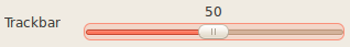
Working with trackbar and named window

The cv2.createTrackbar() method creates a trackbar and takes the following parameters:

Name
Window_name
Value
Count
Onchange()


import numpy as np
import cv2

def empty(z):
    pass

# Create a black background
image = np.zeros((300,512,3), np.uint8)
cv2.namedWindow('Palette')

# create trackbars for colors and associate those with the created window Pallete
cv2.createTrackbar('B','Palette',0,255,empty)
cv2.createTrackbar('G','Palette',0,255,empty)
cv2.createTrackbar('R','Palette',0,255,empty)

while(True):
    cv2.imshow('Palette',image)
    if cv2.waitKey(1) == 27:
        break

    # fetch the color value
    blue = cv2.getTrackbarPos('B','Palette')
    green = cv2.getTrackbarPos('G','Palette')
    red = cv2.getTrackbarPos('R','Palette')
    image[:] = [blue,green,red]

cv2.destroyWindow('Pallete')

The empty() function does not performe any activity when the slider is changed. The cv2.getTrackbarPos() function returns the current position of the specified trackbar. A color palette based on the positions selected repeatedly until a key is pressed, ending the infinite loop and stopping the program.

Working with a webcam

Rather than using the Raspberry Pi camera module, you can use a standard USB webcam to take pictures and video on the Raspberry Pi. The list of supported webcams by Pi at http://elinux.org/RPi_USB_Webcams. Attach your USB webcam to Raspberry Pi through the USB port on Pi and run the lsusb command to make sure it can be listed. Install the fswebcam utility with the command:


   sudo apt-get install fswebcam

You can use the following command to capture the image:


  fswebcam -r 1280x960 --no-banner ~/book/output/camtest.jpg

-r
--no-banner

To record live videos using avconv, install it:


  sudo apt-get install avconv

Use the following command to record a video:


  avconv -f video4linux2 -r 25 -s 544x288 -i /dev/video0 ~/book/output/VideoStream.avi

We can play the video using omxplayer.

Working with a USB webcam using OpenCV


import cv2

# initialize the camera
cam = cv2.VideoCapture(1) # if the video device index is 1 for the Webcam
ret, image = cam.read()

if ret:
    cv2.imshow('videoCaptureTest',image)
    cv2.waitKey(0)
    cv2.destroyWindow('videoCaptureTest')
    cv2.imwrite('videoCaptureTest.jpg',image)

# When everything done, release the capture
cam.release()

You can find out the number of cameras and associated device indexes by using the ls -l /dev/video* command. If the image capture is successful, then cam.read() returns True; otherwise, it will return false. To display a live video stream from a webcam:


import cv2

cam = cv2.VideoCapture(1)
print("Default Resolution is %s x %s\n",  str(int(cam.get(3))) ,str(int(cam.get(4))) )
w=1024
h=768
cam.set(3,w)
cam.set(4,h)

print("Now resolution is set to %x x \n", str(w),str(h) )
while(True):
    # Capture frame-by-frame
    ret, frame = cam.read()
    # Display the resulting frame
    cv2.imshow('Video Test',frame)
    # Wait for Escape Key
    if cv2.waitKey(1) == 27 :
        break


# When everything done, release the capture
cam.release()
cv2.destroyAllWindows()

You can access the features of the video device with cam.get(propertyID). 3 stands for width and 4 stands for height. These properties could be set with cam.set(propertyID, value). To write a video to a file:


 import cv2

cap = cv2.VideoCapture(1)
w=640
h=480
cap.set(3,w)
cap.set(4,h)

# Define the codec and create VideoWriter object
fourcc = cv2.VideoWriter_fourcc(*'XVID')
# frame size in out.write(frame) must be the same as the size argument in the constructor VideoWriter.
out = cv2.VideoWriter('output.avi',fourcc, 20.0, (w,h))

while (cap.isOpened()):
    ret, frame = cap.read()
    if ret == True:
        # write the flipped frame
        out.write(frame)
        cv2.imshow('VideoStream', frame )
        if cv2.waitKey(1) == 27 :
            break 
    else:
        break

# When everything done, release the capture
cap.release()
out.release()
cv2.destroyAllWindows()

cv2.VideoWriter() accepts the following parameters:

Filename
FourCC
Framerate
Resolution

The preceding code records the video until the Esc key is pressed and saves it in the specified file.

Using "with as" in Python 3 (2.6)

Context managers allow you to allocate and release resources precisely when you want to. The most widely used example of context managers is the with statement.


with open('some_file', 'w') as opened_file:
    opened_file.write('Hola!')

The above code opens the file, writes some data to it and then closes it. If an error occurs while writing the data to the file, it tries to close it. The above code is equivalent to:


file = open('some_file', 'w')
try:
    file.write('Hola!')
finally:
    file.close()

The main advantage of using a with statement is that it makes sure our file is closed without paying attention to how the nested block exits.

Working with the Pi camera module

picamera is a python package which provides a programming interface to the Pi camera module. You can install it using

sudo apt-get install python-picamera

To capture a picture,


   import picamera
   import time

   with picamera.PiCamera() as cam:
     cam.resolution=(1024,768)
     cam.start_preview()
     time.sleep(5) # waits for 5 seconds before cam. capture() captures and saves the image in the specified file.
     cam.capture('/home/pi/still.jpg')


   import picamera
   import picamera.array
   import time
   import cv2

   with picamera.PiCamera() as camera:
     rawCap=picamera.array.PiRGBArray(camera)
     camera.start_preview()
     time.sleep(3)
     camera.capture(rawCap,format="bgr")
     image=rawCap.array

   cv2.imshow("Test",image)
   cv2.waitKey(0)
   cv2.destroyAllWindows()

3 Basic Image Processing

Retrieving image properties


   import cv2

   img = cv2.imread('/home/pi/book/test_set/lena_color_512.tif',1)
   print img.shape
   print img.size
   print img.dtype

Arithmetic operations on images

Images are represented as matrices in OpenCV
Images must be of the same size for you to perform arithmetic operations on the images
these operations are performed on individual pixels

cv2.add()
cv2.subtract()

Blending and transitioning images

The cv2.addWeighted(img1, alpha, img2, beta, gamma) function calculates the weighted sum of two images. The output image value is calculated with the following formula:


Output = (alpha*img1) + (beta*img 2) + gamma

We can create a film-style transition effect on the two images by using the same function.


   import cv2
   import numpy as np
   import time

   img1 = cv2.imread('/home/pi/book/test_set/4.2.03.tiff',1)
   img2 = cv2.imread('/home/pi/book/test_set/4.2.04.tiff',1)
   for i in np.linspace(0,1,40):
     alpha=i
     beta=1-alpha
     print 'ALPHA ='+ str(alpha)+' BETA ='+str (beta)
     cv2.imshow('Image Transition', cv2.addWeighted(img1,alpha,img2,beta,0))
     time.sleep(0.05)
     if cv2.waitKey(1) == 27 :
       break
   cv2.destroyAllWindows()

linspace(start, stop, num=50, endpoint=True, retstep=False, dtype=None): Return evenly spaced numbers over a specified interval. Returns num evenly spaced samples, calculated over the interval [start, stop]. The endpoint of the interval can optionally be excluded.

Splitting and merging image colour channels

cv2.split() is used to split an image into three different intensity arrays for each color channel, whereas cv2.merge() is used to merge different arrays into a single multi-channel array, that is, a color image.


   import cv2
   img = cv2.imread('/home/pi/book/test_set/4.2.03.tiff',1)

   b,g,r = cv2.split (img)
   img=cv2.merge((b,g,r))

Creating a negative of an image

A pixel value ranges from 0 to 255, and therefore, negation involves the subtracting of the pixel value from 255.


   import cv2
   img = cv2.imread('/home/pi/book/test_set/4.2.07.tiff')
   grayscale = cv2.cvtColor(img,cv2.COLOR_BGR2GRAY)
   negative = abs(255-grayscale)

Logical operations on images

OpenCV provides bitwise logical operation functions for images.


   import cv2
   import matplotlib.pyplot as plt

   img1 = cv2.imread('/home/pi/book/test_set/Barcode_Hor.png',0)
   img2 = cv2.imread('/home/pi/book/test_set/Barcode_Ver.png',0)

   not_out=cv2.bitwise_not(img1)
   and_out=cv2.bitwise_and(img1,img2)
   or_out=cv2.bitwise_or(img1,img2)
   xor_out=cv2.bitwise_xor(img1,img2)

   titles = ['Image 1','Image 2','Image 1 NOT','AND','OR','XOR']
   images = [img1,img2,not_out,and_out,or_out,xor_out]
   for i in xrange(6):
       plt.subplot(2,3,i+1)
       plt.imshow(images[i],cmap='gray')
       plt.title(titles[i])
       plt.xticks([]),plt.yticks([])
   plt.show()

The xrange type is an immutable sequence object, range creates a list, The plt.subplot() function is used to display multiple images. Typical call signature:


subplot(nrows, ncols, plot_number)

Where nrows and ncols are used to notionally split the figure into nrows * ncols sub-axes, and plot_number is used to identify the particular subplot that this function is to create within the notional grid. plot_number starts at 1, increments across rows first and has a maximum of nrows * ncols. In the preceding example, we created a grid with 2 rows and 3 columns for our images and displayed each image in every part of the grid. In the case when nrows, ncols and plot_number are all less than 10, a convenience exists, such that the a 3 digit number can be given instead, where the hundreds represent nrows, the tens represent ncols and the units represent plot_number. For instance:


subplot(211)

produces a subaxes in a figure which represents the top plot (i.e. the first) in a 2 row by 1 column notional grid.

Colorspaces, Transformations, and Thresholds

Colorspaces and conversions

OpenCV's default colorspace

RGB
Grayscale
HSV

matplotlib uses the RGB format for images so that we need to convert an image from BGR to RGB colorspace before displaying an image with matplotlib. OpenCV has a function cv2.cvtColor(img,conv_flag) that allows us to change the colorspace of an image (img), while the source and target colorspaces are indicated on the conv_flag parameter. For BGR to Gray conversion we use the flags cv2.COLOR_BGR2GRAY. Similarly for BGR to HSV, we use the flag cv2.COLOR_BGR2HSV. To get other flags, just run following commands in your Python terminal :


flags = [i for i in dir(cv2) if i.startswith('COLOR_')]
  print flags

There are 176 Colorspace Conversion flags in OpenCV.

Tracking in real time based on color

In HSV format, it's much easier to recognize the color range.

Hue is expressed as a number from 0 to 360 degrees representing hues of red (which start at 0), yellow (starting at 60), green (starting at 120), cyan (starting at 180), blue (starting at 240) and magenta (starting at 300).
Saturation is the amount of gray from zero percent to 100 percent in the color.
Value (or brightness) works in conjunction with saturation and describes the brightness or intensity of the color from zero percent to 100 percent.

For HSV, Hue range is [0,179], Saturation range is [0,255] and Value range is [0,255]. Different softwares use different scales. So if you are comparing OpenCV values with them, you need to normalize these ranges. We can use the cv2.inRange() function to check whether the part of that image falls within the HSV color range of our interest.


  dst = cv2.inRange(InputArray src, InputArray lowerb, InputArray upperb)

Checks if array elements lie between the elements of two other arrays. dst is set to 255 (all 1 bits) if src is within the specified 1D, 2D, 3D, ... box and 0 otherwise. You can define the pixel in HSV range for tracking:


  mask = cv2.inRange(hsv_img, lower_hsv, upper_hsv)

If the pixel value falls in the given color range, the corresponding pixel in the output image is 255; otherwise it is 0, thus creating a binary mask. How to find HSV values to track? You can use the function cv2.cvtColor(), you just pass the BGR values you want. For example, to find the HSV value of Green, try following commands in Python terminal:


>>> green = np.uint8([[[0,255,0 ]]])
>>> hsv_green = cv2.cvtColor(green,cv2.COLOR_BGR2HSV)
>>> print hsv_green
[[[ 60 255 255]]]

Now you take [H-10, 100,100] and [H+10, 255, 255] as lower bound and upper bound respectively. We can use bitwise_and() to extract the color range we're interested in using this binary mask thereafter.


import numpy as np
import cv2

img=cv2.imread('/home/pi/png.png')
hsv=cv2.cvtColor(img, cv2.COLOR_BGR2HSV)

# blue=np.uint8([[[0,0,255]]])
# hsv_blue=cv2.cvtColor(blue, cv2.COLOR_RGB2HSV)
# print hsv_blue
# [[[120 255 255]]]

lower_blue=np.array([80, 50, 50])
upper_blue=np.array([140, 255, 255])
mask = cv2.inRange(hsv, lower_blue, upper_blue)

cv2.imshow('mask', mask)
cv2.waitKey(0)

tracked=cv2.bitwise_and(img,img,mask=mask)
cv2.imshow('tracked', tracked)
cv2.waitKey(0)

Image transformations

Scaling

Scaling is just resizing of the image. OpenCV comes with a function cv2.resize() for this purpose.



cv2.resize(src, dst [, dsize[, fx[, fy[, interpolation] ] ] ] )

src
dst
dsize
fx
fy
interpolation

INTER_NEAREST - a nearest-neighbor interpolation
INTER_LINEAR - a bilinear interpolation (used by default)
INTER_AREA - resampling using pixel area relation. It may be a preferred method for image decimation, as it gives moire’-free results. But when the image is zoomed, it is similar to the INTER_NEAREST method.
INTER_CUBIC - a bicubic interpolation over 4x4 pixel neighborhood
INTER_LANCZOS4 - a Lanczos interpolation over 8x8 pixel neighborhood

The size of the image can be specified manually, or you can specify the scaling factor. Different interpolation methods are used. Preferable interpolation methods are cv2.INTER_AREA for shrinking and cv2.INTER_CUBIC (slow) & cv2.INTER_LINEAR for zooming. By default, interpolation method used is cv2.INTER_LINEAR for all resizing purposes. You can resize an input image either of following methods:


import cv2
import numpy as np

img = cv2.imread('messi5.jpg')
res = cv2.resize(img,None,fx=2, fy=2, interpolation = cv2.INTER_CUBIC)
#OR
height, width = img.shape[:2]
res = cv2.resize(img,(2*width, 2*height), interpolation = cv2.INTER_CUBIC)

The following example shows the usage for upscaling and downscaling:


   import cv2

   img = cv2.imread('/home/pi/book/test_set/house.tiff',1)
   upscale = cv2.resize(img,None,fx=1.5,fy=1.5,interpolation=cv2.INTER_CUBIC)
   downscale = cv2.resize(img,None,fx=0.5,fy=0.5, interpolation=cv2.INTER_AREA)
   cv2.imshow('upscale',UpScale)
   cv2.waitKey(0)
   cv2.imshow('downscale',DownScale)
   cv2.waitKey(0)
   cv2.destroyAllWindows()

Translation, rotation, and affine transformation

The cv2.warpAffine() function can be used to perform translation, rotation, and affine transformation. OpenCV provides two transformation functions, cv2.warpAffine and cv2.warpPerspective, with which you can have all kinds of transformations. cv2.warpAffine takes a 2x3 transformation matrix while cv2.warpPerspective takes a 3x3 transformation matrix as input.

Translation


1 0 Tx
0 1 Ty


rows,cols = img.shape
M = np.float32([[1,0,100],[0,1,50]])
dst = cv2.warpAffine(img, M ,(cols,rows))

Rotations

getRotationMatrix2D


rows,cols,channel = img.shape
   R = cv2.getRotationMatrix2D((cols/2,rows/2),45,0.5)
   output = cv2.warpAffine(input,R,(cols,rows))

Affine transformations

getAffineTransform

warpAffine


   points1 = np.float32([[100,100],[300,100],[100,300]])
   points2 = np.float32([[200,150],[400,150],[100,300]])
   A = cv2.getAffineTransform(points1,points2)
   output = cv2.warpAffine(input,A,(cols,rows))

Perspective transformation


import cv2
   import numpy as np
   from matplotlib import pyplot as plt
   image = cv2.imread('/home/pi/book/test_set/ruler.512.tiff',1)
   #changing the colorspace from  BGR->RGB
   input = cv2.cvtColor(image, cv2.COLOR_BGR2RGB )
   rows,cols,channels = input.shape
   points1 = np.float32([[0,0],[400,0],[0,400],[400,400]])
   points2 = np.float32([[0,0],[300,0],[0,300],[300,300]])
   P = cv2.getPerspectiveTransform(points1,points2)
   output = cv2.warpPerspective(input,P,(300,300))
   plt.subplot(121),plt.imshow(input),plt.title('Input')
   plt.subplot(122),plt.imshow(output),plt.title('Perspective Transform')
   plt.show()

Thresholding image

In OpenCV, the cv2.threshold() function is used to threshold images. It takes as input, grayscale image, threshold value, maxVal, and threshold method as parameters, and returns the thresholded image as output. The maxVal parameter is the value assigned to the pixel if the pixel intensity is greater (or less in some methods) than the threshold. There are five threshold methods available in OpenCV:

cv2.THRESH_BINARY
cv2.THRESH_BINARY_INV
cv2.THRESH_TRUNC
cv2.THRESH_TOZERO
cv2.THRESH_TOZERO_INV

Otsu's method

If the image has background and foreground pixels, Otsu's method is the best way to separate these two sets of pixels automatically without specifying the threshold value. This method is applied in addition to other methods and the threshold is passed as 0. Try implementing the following code:


   ret,output=cv2.threshold(image,0,255,cv2.THRESH_BINARY+cv2.THRESH_OTSU)

Noise and filter

Kernels

In image processing, a kernel, convolution matrix, or mask is a small matrix used in some image processing operations. It is used for blurring, sharpening, embossing, edge detection, and more. This is accomplished by doing a convolution between a kernel and an image. Convolution is the process of adding each element of the image to its local neighbors, weighted by the kernel. Depending on the element values, a kernel can cause a wide range of effects. One of the main uses of kernels is to apply a low-pass filter to an image. Low-pass filters average out the rapid changes in the intensity of image pixels. This basically smoothens or blurs the image. A simple averaging kernel can be mathematically represented as follows:


 Ones Matrix / rows * cols

We can use the following NumPy code to create a 3x3 averaging kernel:


   K=np.ones((3,3),np.uint32)/9

numpy.ones(shape, dtype=None, order='C') Return a new array of given shape and type, filled with ones.

2D convolution filtering

Each output pixel is altered by contributions from a number of adjoining input pixels. These types of operations are commonly referred to as convolution or spatial convolution. Convolution kernels typically feature an odd number of rows and columns in the form of a square, with a 3 x 3 pixel mask (convolution kernel) being the most common form, but 5 x 5 and 7 x 7 kernels are also frequently employed.

OpenCV provides a function cv2.filter2D() to convolve a kernel with an image.


cv2.filter2D(src, ddepth, kernel[, dst[, anchor[, delta[, borderType]]]]) → dst¶

where

src
ddepth

src.depth() = CV_8U, ddepth = -1/CV_16S/CV_32F/CV_64F
src.depth() = CV_16U/CV_16S, ddepth = -1/CV_32F/CV_64F
src.depth() = CV_32F, ddepth = -1/CV_32F/CV_64F
src.depth() = CV_64F, ddepth = -1/CV_64F

kernel
dst
anchor
delta
borderType

As an example, we will try an averaging filter on an image. A 5x5 averaging filter kernel is used:


    import cv2
    import numpy as np
    from matplotlib import pyplot as plt
     
    img = cv2.imread('opencv_logo.png')
     
    kernel = np.ones((5,5),np.float32)/25
    dst = cv2.filter2D(img,-1,kernel)
     
    plt.subplot(121),plt.imshow(img),plt.title('Original')
    plt.xticks([]), plt.yticks([])
    plt.subplot(122),plt.imshow(dst),plt.title('Averaging')
    plt.xticks([]), plt.yticks([])
    plt.show()

Low-pass filtering

boxFilter

Blurs an image using the box filter.


dst = cv2.boxFilter(src, ddepth, ksize[, dst[, anchor[, normalize[, borderType]]]])

The cv2.boxFilter() function takes the image, ddepth, and size of the kernel as inputs and blurs the image. We can specify normalize as either true or false. The function smoothes an image using the kernel:

blur

Blurs an image using the normalized box filter.


dst = cv2.blur(src, ksize[, dst[, anchor[, borderType]]])

The call blur(src, dst, ksize, anchor, borderType) is equivalent to boxFilter(src, dst, src.type(), anchor, true, borderType) .

GaussianBlur

Blurs an image using a Gaussian filter.


cv2.GaussianBlur(src, ksize, sigmaX[, dst[, sigmaY[, borderType]]])

The function convolves the source image with the specified Gaussian kernel. This filter is highly effective against Gaussian noise.

medianBlur

Blurs an image using the median filter.


dst = cv2.medianBlur(src, ksize[, dst])

Parameters:

src
ksize
dst

It calculates the median of all the values under the kernel, and the centre pixel in the kernel is replaced with the calculated medium. In this filter, a window slides along the image, and the median intensity value of the pixels within the window becomes the output intensity of the pixel being processed. It's highly effective against salt-and-pepper noise. The following code introduces salt-and-pepper noise in the image and then applies the cv2.medianBlur() function to that to remove the noise:


import cv2
   import numpy as np
   import random
   from matplotlib import pyplot as plt
   img = cv2.imread('/home/pi/book/test_set/lena_color_512.tif',1)
   input = cv2.cvtColor(img,cv2.COLOR_BGR2RGB)
   output = np.zeros(input.shape,np.uint8)
   p = 0.2 # probablity of noise
   for i in range (input.shape[0]):
     for j in range(input.shape[1]):
       r = random.random()
       if r < p/2:
         output[i][j] = 0,0,0
       elif r < p:
         output[i][j] = 255,255,255
       else:
         output[i][j] = input[i][j]
   noise_removed = cv2.medianBlur(output,3)
   plt.subplot(121),plt.imshow(output),plt.title('Noisy Image')
   plt.xticks([]), plt.yticks([])
   plt.subplot(122),plt.imshow(noise_removed),plt.title('Median
   Filtering')
   plt.xticks([]), plt.yticks([])
   plt.show()

Chapter 6 Edges, Circles, and Lines' Detection

High-pass filters

All high-pass filters(HPF) will let high-frequency information like edges to enhance, while restricting low-frequency information (hence, they are called high-pass filters). These filters are also called derivative masks and are widely used in edge detection and extraction algorithms. OpenCV provides three types of gradient filters or High-pass filters:

Sobel()

Vertical direction


-1 0 1
-2 0 2
-1 0 1

Horizontal direction


-1 -2 -1
0 0 0
1 2 1


Sobel  (  InputArray   src,
  OutputArray   dst,
  int   ddepth,
  int   dx,
  int   dy,
  int   ksize = 3,
  double   scale = 1,
  double   delta = 0,
  int   borderType = BORDER_DEFAULT 
 )

src
dst
ddepth
dx
dy
ksize
scale
delta
borderType

Laplacian()

Positive Laplacian Operator


0 1 0
1 -4 1
0 1 0

Negative Laplacian Operator


0 -1 0
-1 4 -1
0 -1 0

Scharr()


Scharr(src, dst, ddepth, dx, dy, scale, delta, borderType)


Sobel(src, dst, ddepth, dx, dy, CV\_SCHARR, scale, delta, borderType).



import cv2
import matplotlib.pyplot as plt


img=cv2.imread('grid.jpg',1)

laplacian = cv2.Laplacian(img,ddepth=cv2.CV_32F, ksize=17,scale=1,delta=0,borderType=cv2.BORDER_DEFAULT)
sobel = cv2.Sobel(img,ddepth=cv2.CV_32F,dx=1,dy=0, ksize=11,scale=1,delta=0,borderType=cv2.BORDER_DEFAULT)
scharr = cv2.Scharr(img,ddepth=cv2.CV_32F,dx=1,dy=0,scale=1,delta=0,borderType=cv2.BORDER_DEFAULT)
sobelx = cv2.Sobel(img,cv2.CV_64F,1,0,ksize=7)
sobely = cv2.Sobel(img,cv2.CV_64F,0,1,ksize=7)
    
images=[img,laplacian,sobel,scharr,sobelx,sobely]
titles=['Original','Laplacian','Sobel','Scharr', 'Sobel-x','Sobel-y']

for i in range(6):
    plt.subplot(3,2,i+1)
    plt.imshow(images[i],cmap = 'gray')
    plt.title(titles[i]), plt.xticks([]), plt.yticks([])

plt.show()

Canny Edge detector

The Canny Edge detector is a multistage edge detection method developed by John Canny:

Noise Reduction
Finding Intensity Gradient of the Image
Non-maximum Suppression
Hysteresis Thresholding

OpenCV puts all the above in single function, cv2.Canny(). The following parameters are usually passed to cv2.Canny() :

image
threshold1
threshold2
apertureSize
L2gradient

accurate L2

The function will return a set with the detected edges; single channels 8-bit image, which has the same size as image .


import cv2
import matplotlib.pyplot as plt
img = cv2.imread('/home/jerry/grid.jpg',0)
edges1 = cv2.Canny(img,100,200,L2gradient=False)
edges2 = cv2.Canny(img,100,200,L2gradient=True)
images = [img,edges1,edges2]
titles = ['Original','L1 Gradient','L2 Gradient']
for i in range(3):
    plt.subplot(1,3,i+1)
    plt.imshow(images[i],cmap = 'gray')
    plt.title(titles[i]),
    plt.xticks([]), plt.yticks([])

plt.show()

Hough circle and line transforms

OpenCV has cv2.HoughCircles() to detect the circle feature in an image, and it returns the circles in the images in the form of a vector (x, y, radius).


import cv2
import numpy as np

img = cv2.imread('/home/jerry/opencv.png',0) # Load an image
img = cv2.medianBlur(img,5) #  to reduce noise and avoid false circle detection
cimg = cv2.cvtColor(img,cv2.COLOR_GRAY2BGR) # Convert it to grayscale

circles = cv2.HoughCircles(img,cv2.HOUGH_GRADIENT,1,20,
                            param1=50,param2=30,minRadius=0,maxRadius=0)

circles = np.uint16(np.around(circles))
for i in circles[0,:]:
    # draw the outer circle
    cv2.circle(cimg,(i[0],i[1]),i[2],(0,255,0),2)
    # draw the center of the circle
    cv2.circle(cimg,(i[0],i[1]),2,(0,0,255),3)

cv2.imshow('detected circles',cimg)
cv2.waitKey(0)
cv2.destroyAllWindows()

To apply Hough Circle Transform with the arguments:

src_gray
CV_HOUGH_GRADIENT
dp
min_dist
param_1
param_2
min_radius
max_radius

This function returns a vector of circles that stores sets of 3 values: (x, y, r) for each detected circle. OpenCV also has a cv2.HoughLines() function to find the lines. To use Hough Lines Transform, processed image should be binary. But we would like to search for the straight lines on an original, color image. Therefore, probably the most common solution is to firstly grayscale the image and then to detect edges. Such mask of edges can be then fetched to the Hough Lines method which should output a set of straight lines found on an image. A line can be represented as y = mx+c (Cartesan coordinate system) or in parametric form (Polar coordinate system), as


     (r, theta)

where r is the perpendicular distance from origin to the line, and theta is the angle formed by this perpendicular line and horizontal axis measured in counter-clockwise (in OPenCV).


  y * sin(theta) + x * cos(theta) = d

Therefore, with a known (d , theta), you can draw a line for a given range for x ( y can be calculated by the above formula). [reference] we can draw such point in (ρ,θ) coordinates which will be later called a Hough space.

Now, in the image space, we are drawing other lines which are intersecting at one common point. Let's see what points will be produced in Hough space which are corresponding to these lines.

It turns out that these points in (ρ,θ) space are forming a sinusoid.

Finally, maybe the most interesting effect. If we draw points which form a line in the image space, we will obtain a bunch of sinusoids in the Hough space. But, magically, they are intersecting at exactly one point!

It means that, to identify candidates for being a straight line, we should seek for intersections in Hough space. Now let’s see how Hough Transform works for lines. Any line can be represented in these two terms, (d, theta). So first it creates a 2D array or accumulator (to hold values of two parameters) and it is set to 0 initially. Let rows denote the d and columns denote the theta. Size of array depends on the accuracy you need. Suppose you want the accuracy of angles to be 1 degree, you need 180 columns. For r, the maximum distance possible is the diagonal length of the image. So taking one pixel accuracy, number of rows can be diagonal length of the image.


import matplotlib.pyplot as plt
import matplotlib.image as mpimg
import numpy as np
import cv2

def draw_lines(img, houghLines, color=[0, 255, 0], thickness=2):
    for line in houghLines:
        for rho,theta in line:
            a = np.cos(theta)
            b = np.sin(theta)
            x0 = a*rho
            y0 = b*rho
            x1 = int(x0 + 1000*(-b))
            y1 = int(y0 + 1000*(a))
            x2 = int(x0 - 1000*(-b))
            y2 = int(y0 - 1000*(a))
 
            cv2.line(img,(x1,y1),(x2,y2),color,thickness)   
                
 
def weighted_img(img, initial_img, α=0.8, β=1., λ=0.):
    return cv2.addWeighted(initial_img, α, img, β, λ)    

 
image = mpimg.imread("licensePlate.jpg")
gray_image = cv2.cvtColor(image, cv2.COLOR_RGB2GRAY)
blurred_image = cv2.GaussianBlur(gray_image, (9, 9), 0)
edges_image = cv2.Canny(blurred_image, 50, 120)
   
rho_resolution = 1
theta_resolution = np.pi/180
threshold = 155
 
hough_lines = cv2.HoughLines(edges_image, rho_resolution , theta_resolution , threshold)
 
hough_lines_image = np.zeros_like(image)
draw_lines(hough_lines_image, hough_lines)
original_image_with_hough_lines = weighted_img(hough_lines_image,image)
 
plt.figure(figsize = (30,20))
plt.subplot(131)
plt.imshow(image)
plt.subplot(132)
plt.imshow(edges_image, cmap='gray')
plt.subplot(133)
plt.imshow(original_image_with_hough_lines, cmap='gray') 
plt.show()

It's worth noting that in OpenCV there exists another version of the function to find Hough Lines. It's named HoughLinesP. P suffix stands for probabilistic here. It doesn’t take all the points into consideration, instead take only a random subset of points and that is sufficient for line detection. Just we have to decrease the threshold. The Hough transform functions have to be tuned for the given sample set. So, if you cannot see any circles and lines in your video or if there are a lot of false positives (that is, the programs detect circles and lines even when they are not present in the input frame), you might want to play a bit with the parameters to tune them according to your sample input to get the desired results. OpenCV implementation is based on Robust Detection of Lines Using the Progressive Probabilistic Hough Transform by Matas, J. and Galambos, C. and Kittler, J.V.. The function used is cv2.HoughLinesP(). It has two new arguments.

minLineLength
maxLineGap

Best thing is that, it directly returns the two endpoints of lines.


import cv2
import numpy as np

img = cv2.imread('dave.jpg')
gray = cv2.cvtColor(img,cv2.COLOR_BGR2GRAY)
edges = cv2.Canny(gray,50,150,apertureSize = 3)
minLineLength = 100
maxLineGap = 10
lines = cv2.HoughLinesP(edges,1,np.pi/180,100,minLineLength,maxLineGap)
for x1,y1,x2,y2 in lines[0]:
    cv2.line(img,(x1,y1),(x2,y2),(0,255,0),2)

cv2.imwrite('houghlines5.jpg',img)

Chapter 7 Image Restoration, Quantization, and Depth Map

Restoring images using inpainting

Image restoration is the process of reconstructing the damaged parts of an image. OpenCV offers two of these with its cv2.inpaint() function. It accepts a source image, an inpaint mask that is a grayscale image representation of the damaged area where the nonzero (white) pixels denote the area to be inpainted, an inpaint neighborhood side, and an algorithm ( cv2.INPAINT_TELEA, cv2.INPAINT_NS )that has to be applied as parameters. The function then returns the inpainted image. We need to create a mask of same size as that of input image, where non-zero pixels corresponds to the area which is to be inpainted.


import numpy as np
import cv2
img = cv2.imread('messi_2.jpg')
mask = cv2.imread('mask2.png',0)
dst = cv2.inpaint(img,mask,3,cv2.INPAINT_TELEA)
cv2.imshow('dst',dst)
cv2.waitKey(0)
cv2.destroyAllWindows()

Image segmentation

Image segmentation is the process of dividing images into multiple, relevant sections or parts based on some criteria. Thresholding the image can be considered the simplest form of segmentation.

Mean shift algorithm based segmentation

PyMeanShift is a Python module/extension for segmenting images using the mean shift algorithm. The mean shift algorithm and its C++ implementation are by Chris M. Christoudias and Bogdan Georgescu. The PyMeanShift extension provides a Python interface to the meanshift C++ implementation using Numpy arrays. Installation instructions :

Download the latest version from https://github.com/fjean/pymeanshift/archive/master.zip
Decompress the file then run the following commands to build and install it
vefify the installation

If you see the build error "fatal error: Python.h: No such file or directory", you deed to install phytho3-devel package.


   sudo dnf install python3-devel

An example,


import cv2
import pymeanshift as pms
from matplotlib import pyplot as plt

original_image = cv2.imread("licensePlate.jpg")
#changing the colorspace from BGR->RGB
input_image = cv2.cvtColor(original_image, cv2.COLOR_BGR2RGB )

(segmented_image, labels_image, number_regions) = pms.segment(input_image, spatial_radius=6, range_radius=4.5, min_density=50)

plt.subplot(131),plt.imshow(input_image),plt.title('input_image')
plt.xticks([]),plt.yticks([])
plt.subplot(132),plt.imshow(segmented_image),plt.title(
'Segmented Output')
plt.xticks([]),plt.yticks([])
plt.subplot(133),plt.imshow(labels_image),plt.title(
'Labeled Output')
plt.xticks([]),plt.yticks([])
plt.show()

K-means clustering and image quantization

The k-means clustering algorithm is a quantization algorithm that maps sets of values within a range into a cluster determined by a value (mean). It basically divides a given set of n values into k partitions. This is called clustering when it's applied on data with two or more dimensions. OpenCV has cv2.kmeans() for the implementation of the k-means algorithm. It accepts the following input parameters:

samples
nclusters(K)
criteria

type of termination criteria
max_iter
epsilon

attempts
flags

Output parameters

compactness
labels
centers

Consider data with Only One Feature,


import numpy as np
import cv2
from matplotlib import pyplot as plt

x = np.random.randint(25,100,25)
y = np.random.randint(175,255,25)
z = np.hstack((x,y)) # Stack arrays in sequence horizontally (column wise).
z = z.reshape((50,1))
z = np.float32(z)
plt.hist(z,256,[0,256])
plt.show()

So we have ‘z’ which is an array of size 50,

values ranging from 0 to 255
'z' is reshaped to a column vector for 1 feature

Now we apply the KMeans function.


# whenever 10 (max_iter) iterations of algorithm is ran, or an accuracy of 1.0 (epsilon)is reached, stop the algorithm and return the answer
criteria = (cv2.TERM_CRITERIA_EPS + cv2.TERM_CRITERIA_MAX_ITER, 10, 1.0)

# Set flags (Just to avoid line break in the code)
flags = cv2.KMEANS_RANDOM_CENTERS

# Apply KMeans
compactness,labels,centers = cv2.kmeans(z,2,None,criteria,10,flags)

In this case, we got 2 centers.

>>> centers
array([[  63.47999954],
       [ 213.24000549]], dtype=float32)

Labels will have the same size as that of test data where each data will be labelled as ‘0’,‘1’,‘2’ etc. depending on their centroids. Now we split the data to different clusters depending on their labels. Now we split the data to different clusters depending on their labels.


A = z[labels==0]
B = z[labels==1]

Now we plot A in Red color and B in Blue color and their centroids in Yellow color.


# Now plot 'A' in red, 'B' in blue, 'centers' in green
plt.hist(A,256,[0,256],color = 'r')
plt.hist(B,256,[0,256],color = 'b')
plt.hist(centers,32,[0,256],color = 'g')
plt.show()

Consider data with Multiple Features, each feature is arranged in a column, while each row corresponds to an input test sample. Here is an example for 2 features


import numpy as np
import cv2
from matplotlib import pyplot as plt

# create two 25 x 2  matrixes
X = np.random.randint(25,50,(25,2))
Y = np.random.randint(60,85,(25,2))
Z = np.vstack((X,Y))

# convert to np.float32
Z = np.float32(Z)

# define criteria and apply kmeans()
criteria = (cv2.TERM_CRITERIA_EPS + cv2.TERM_CRITERIA_MAX_ITER, 10, 1.0)
ret,label,center=cv2.kmeans(Z,2,None,criteria,10,cv2.KMEANS_RANDOM_CENTERS)

# Now separate the data. Note the ravel() return a contiguous flattened (1-D) array.
A = Z[label.ravel()==0]
B = Z[label.ravel()==1]

# Plot the data. Make a scatter plot of (x,y).
plt.scatter(A[:,0],A[:,1])
plt.scatter(B[:,0],B[:,1],c = 'r')
plt.scatter(center[:,0],center[:,1],s = 80,c = 'y', marker = 's')
plt.xlabel('Height'),plt.ylabel('Weight')
plt.show()

In this case, we got 2 centers.

>>> center
array([[ 72.48000336,  72.31999969],
       [ 36.15999985,  34.91999817]], dtype=float32)

Color Quantization is the process of reducing number of colors in an image. There are 3 features, say, R,G,B. So we need to reshape the image to an array of Mx3 size (M is number of pixels in image).


import cv2
import numpy as np
import matplotlib.pyplot as plt

image=cv2.imread('licensePlate.jpg')
input = cv2.cvtColor(image,cv2.COLOR_BGR2RGB)
Z=input.reshape((-1,3))
Z=np.float32(Z)
criteria=(cv2.TERM_CRITERIA_EPS+ cv2.TERM_CRITERIA_MAX_ITER,10,1.0)

K=2
ret,label1,center1=cv2.kmeans(Z,K, None,criteria,10,cv2.KMEANS_RANDOM_CENTERS)
center1=np.uint8(center1)
res1=center1[label1.flatten()]
output1=res1.reshape((image.shape))

K=4
ret,label2,center2=cv2.kmeans(Z,K,None,criteria,10,cv2.KMEANS_RANDOM_CENTERS)
center2=np.uint8(center2)
res2=center2[label2.flatten()]
output2=res2.reshape((image.shape))

K=8
ret,label3,center3=cv2.kmeans(Z,K,None,criteria,10,cv2.KMEANS_RANDOM_CENTERS)

# Now convert back into uint8, and make original image
center3=np.uint8(center3)
res3=center3[label3.flatten()]
output3=res3.reshape((image.shape))
titles=['Original','K=2','K=4','K=8']
output=[input,output1,output2,output3]
for i in range(4):
    plt.subplot(2,2,i+1),plt.imshow(output[i]),plt.title(titles[i])
    plt.xticks([]),plt.yticks([])
    
plt.show()

Disparity map and depth estimation

Disparity refers to the difference in the location of an object in the corresponding two (left and right) images as seen by the left and right eye, which is created due to a parallax. Our brain uses this disparity to estimate the depth information from the pair of two-dimensional images. In biology, this is called stereoscopic vision. OpenCV provides the cv2.StereoBM.compute() function, which takes the left image and the right image as a parameter and returns the disparity map of the image pair.


import numpy as np
import cv2
from matplotlib import pyplot as plt

# Load the left and right images in gray scale
imgL = cv2.imread('tsukuba_l.png',0)
imgR = cv2.imread('tsukuba_r.png',0)
# Initialize the stereo block matching object 
stereo = cv2.StereoBM_create(numDisparities=32, blockSize=13)
# Compute the disparity image
disparity = stereo.compute(imgL,imgR)

titles=['Left','Right','Depth Map']
output=[imgL,imgR,disparity]
for i in xrange(3):
 plt.subplot(1,3,i+1),plt.imshow(output[i],cmap='gray')
 plt.title(titles[i])
 plt.xticks([]),plt.yticks([])
plt.show()

Chapter 8 Histograms, Contours, Morphological Transformations, and Performance Measurement

Image histograms

A histogram is a way to graphically represent the distribution of data. the histogram of an image is a graphical representation of the distribution of color or luminance variance in an image. Both OpenCV and Numpy come with in-built function for histogram. Matplotlib comes with a histogram plotting function : matplotlib.pyplot.hist()

matplotlib.pyplot.hist(
    x, bins=None, range=None, normed=False, weights=None, cumulative=False, bottom=None, histtype='bar', align='mid', orientation='vertical', rwidth=None, log=False, color=None, label=None, stacked=False, hold=None, data=None, **kwargs
  )

Parameters:

x
bins
range


import cv2
import matplotlib.pyplot as plt
img = cv2.imread('/home/pi/book/test_set/4.1.08.tiff',0)
plt.hist(img.ravel(),256,[0,256])
plt.show()

.ravel(), is an attribute to numpy matrices, which can be used to faltten the src Matrix, there are other similar APIs' as well which can be used for this purpose such as : .flatten(), .reshape() The NumPy library also has an np.histogram() histogram function that can be used to compute the histogram of a set of data.


 hist, bin_edges = numpy.histogram(a, bins=10, range=None, normed=False, weights=None, density=None)

OpenCV also has a function to compute histograms for color images.


  cv2.calcHist(images, channels, mask, histSize, ranges[, hist[, accumulate]])

images : it is the source image of type uint8 or float32. it should be given in square brackets, ie, "[img]".
channels : it is also given in square brackets. It is the index of channel for which we calculate histogram. For example, if input is grayscale image, its value is [0]. For color image, you can pass [0], [1] or [2] to calculate histogram of blue, green or red channel respectively.
mask : mask image. To find histogram of full image, it is given as "None". But if you want to find histogram of particular region of image, you have to create a mask image for that and give it as mask. (I will show an example later.)
histSize : this represents our BIN count. Need to be given in square brackets. For full scale, we pass [256].
ranges : this is our RANGE. Normally, it is [0,256].

The following example shows its usage by plotting a histogram for each channel (red, green, and blue):


import cv2
from matplotlib import pyplot as plt

img = cv2.imread('building.jpg',1)
input=cv2.cvtColor(img,cv2.COLOR_RGB2BGR)
histr_RED = cv2.calcHist([input],[0],None,[256],[0,256])
histr_GREEN = cv2.calcHist([input],[1],None,[256],[0,256])
histr_BLUE = cv2.calcHist([input],[2],None,[256],[0,256])
plt.subplot(221),plt.imshow(input),plt.title('Original
Image'),plt.xticks([]),plt.yticks([])
plt.subplot(222),plt.plot(histr_RED,color='r'),
plt.title('Red'), plt.xlim([0,256]), plt.yticks([])
plt.subplot(223),plt.plot(histr_GREEN,color='g'), plt.title('Green'),
plt.xlim([0,256]), plt.yticks([])
plt.subplot(224),plt.plot(histr_BLUE,color='b'), plt.title('Blue'),
plt.xlim([0,256]), plt.yticks([])
plt.show()

Image contours

A contour is a curve joining all the continuous points along the boundary with the same color value. Contours are often obtained from edges, but they are aimed to be object contours For better accuracy, use binary images. So before finding contours, apply threshold or canny edge detection. In OpenCV, finding contours is like finding white object from black background. So remember, object to be found should be white and background should be black.


import numpy as np
import cv2
import matplotlib.pyplot as plt

im = cv2.imread('licensePlate.jpg')
imgray = cv2.cvtColor(im, cv2.COLOR_BGR2GRAY)
ret, thresh = cv2.threshold(imgray, 127, 255, 0)
im2, contours, hierarchy = cv2.findContours(thresh, cv2.RETR_TREE, cv2.CHAIN_APPROX_SIMPLE)

cv2.drawContours(im, contours, -1, (0,255,0), 3)
plt.imshow(im)
plt.title('Contours')
plt.xticks([])
plt.yticks([])
plt.show()

If you need to draw a specific contour,then you can use cv2.drawContours by specifying the contour index.


  cv2.drawContours(im, contours, 100, (0,255,0), 3)

Morphological transformations on image

Morphological transformations are some simple operations based on the image shape. It is normally performed on binary images. It needs two inputs, one is our original image, second one is called structuring element or kernel which decides the nature of operation. Two basic morphological operators are Erosion and Dilation. Then its variant forms like Opening, Closing, Gradient etc also comes into play.

Erosion(侵蝕)

keep foreground in white

Dilation(擴張)
morphological Opening


opening = cv2.morphologyEx(img, cv2.MORPH_OPEN, kernel)

morphological Closing


  closing = cv2.morphologyEx(img, cv2.MORPH_CLOSE, kernel)

morphological Gradient


import numpy as np
import cv2
from matplotlib import pyplot as plt

img = cv2.imread('blackWhite.png',0)
kernel = np.ones((5,5),np.uint8)
erosion = cv2.erode(img,kernel,iterations = 2)
dilation = cv2.dilate(img,kernel,iterations = 2)
gradient = cv2.morphologyEx(img, cv2.MORPH_GRADIENT, kernel)
titles=['Original','Erosion','Dilation','Gradient']
output=[img,erosion,dilation,gradient]

for i in range(4):
    plt.subplot(2,2,i+1),plt.imshow(output[i],cmap='gray')
    plt.title(titles[i]),plt.xticks([]),plt.yticks([])

plt.show()

We manually created a structuring elements in the previous examples with help of Numpy. It is rectangular shape. But in some cases, you may need elliptical/circular shaped kernels. So for this purpose, OpenCV has a function, cv2.getStructuringElement(). You just pass the shape and size of the kernel, you get the desired kernel.


# Rectangular Kernel
>>> cv2.getStructuringElement(cv2.MORPH_RECT,(5,5))
array([[1, 1, 1, 1, 1],
       [1, 1, 1, 1, 1],
       [1, 1, 1, 1, 1],
       [1, 1, 1, 1, 1],
       [1, 1, 1, 1, 1]], dtype=uint8)

# Elliptical Kernel
>>> cv2.getStructuringElement(cv2.MORPH_ELLIPSE,(5,5))
array([[0, 0, 1, 0, 0],
       [1, 1, 1, 1, 1],
       [1, 1, 1, 1, 1],
       [1, 1, 1, 1, 1],
       [0, 0, 1, 0, 0]], dtype=uint8)

# Cross-shaped Kernel
>>> cv2.getStructuringElement(cv2.MORPH_CROSS,(5,5))
array([[0, 0, 1, 0, 0],
       [0, 0, 1, 0, 0],
       [1, 1, 1, 1, 1],
       [0, 0, 1, 0, 0],
       [0, 0, 1, 0, 0]], dtype=uint8)

OpenCV performance measurement and improvement

In Python, we can use the time library to obtain the current time. This allows us to measure how long a piece of code takes to run, as shown in the following code:


t1 = time.time()
# Image Processing code goes here
t2 = time.time()
print (t2-t1)

OpenCV also provides cv2.getTickCount() and cv2.getTickFrequency() , which can be used for the same purpose. The cv2.getTickCount() function returns the number of clock cycles and cv2.getTickFrequency() returns the clock frequency.


c1=cv2.getTickCount()
# Image processing code goes here
c2=cv2.getTickCount()
print ((c2-c1)/cv2.getTickFrequency())

Chapter 9 Real-life Computer Vision Applications

Barcode detection

A barcode always has a very high horizontal gradient and a very low vertical gradient. So, in our image, we need to search for a region that fulfills this property.


import numpy as np
import cv2

image=cv2.imread('barcode.jpg',1)
input = cv2.cvtColor(image, cv2.COLOR_BGR2GRAY)
cv2.imshow('input', input)
cv2.waitKey(0)

The best way to accomplish this is to compute the Sobel derivatives of the first order in horizontal and vertical directions, and then subtract the vertical derivative from the horizontal derivative


hor_der = cv2.Sobel(input, ddepth = -1 , dx = 1, dy = 0, ksize=5)
ver_der = cv2.Sobel(input, ddepth = -1 , dx = 0, dy = 1, ksize=5)
diff = cv2.subtract(hor_der, ver_der)
diff = cv2.convertScaleAbs(diff)
cv2.imshow('diff', diff)
cv2.waitKey(0)

We convert the output in 8-bit unsigned integer format using:


 cv.ConvertScaleAbs(src, dst, scale=1.0, shift=0.0)

On each element of the input array, the function convertScaleAbs performs three operations sequentially: scaling, taking an absolute value, conversion to an unsigned 8-bit type:


 dst = (unsigned char) src * scale + shift

Then we can apply Gaussian blur and a binary threshold to this blurred image with 255


blur = cv2.GaussianBlur(diff, (3, 3),0)
ret, th = cv2.threshold(blur, 225, 255, cv2.THRESH_BINARY)

This will yield the following image:

We can fill in the gaps between the bars of the barcode by dilating it:


dilated = cv2.dilate(th, None, iterations = 7)

The output will contain a big rectangle-like box corresponding to the barcode region.

We can eliminate the other region that we're not interested in with the erosion operation:


eroded = cv2.erode(dilated, None, iterations = 7)

We can find out the list of contours in this binary image then the biggest contour in this image would be the contour corresponding to the barcode region.


_, contours, _ = cv2.findContours(eroded, cv2.RETR_TREE,cv2.CHAIN_APPROX_SIMPLE)
areas = [cv2.contourArea(temp) for temp in contours]
max_index = np.argmax(areas)
largest_contour=contours[max_index]

We can get the coordinates of the bounding rectangle for the contour with cv2.boundingRect() , an OpenCV function, and draw it as follows:


x,y,width,height = cv2.boundingRect(largest_contour)
cv2.rectangle(image,(x,y),(x+width,y+height),(0,255,0),2)
cv2.imshow('Detected Barcode',image)
cv2.waitKey(0)
cv2.destroyAllWindows()

Note, the iterations used in dilate() and erode() need to be tuned for different images to get the best effect. Use the same image to be tested for different iterations:

"iterations=15"

"iterations=4"

Motion detection and tracking



import cv2
import numpy as np

camera = cv2.VideoCapture(1)

# create a kernel for the dilation operation,
k=np.ones((3,3),np.uint8)

# initialize the first frame
f1_gray = None

while(True):
    # grab the current frame
    (grabbed, f2) = camera.read()
    # if the frame could not be grabbed, end it.
    if not grabbed:
        break
    
    # convert it to grayscale, and blur it
    f2_gray = cv2.cvtColor(f2, cv2.COLOR_BGR2GRAY)
    f2_gray = cv2.GaussianBlur(f2_gray, (21, 21), 0)

    # if the first frame has not set, initialize it
    if f1_gray is None:
        f1_gray = f2_gray
        continue

    # compute the absolute difference between the current frame and the last frame
    frameDelta = cv2.absdiff(f1_gray, f2_gray) 
    # convert this noise-removed output into a binary image
    ret, th = cv2.threshold(frameDelta, 25, 255, cv2.THRESH_BINARY)
    # dilate the image so that it is easier for us to find the boundary clearly
    dilated=cv2.dilate(th, k, iterations=2)
    # find the contour
    im2, contours, hierarchy= cv2.findContours(dilated, cv2.RETR_TREE, cv2.CHAIN_APPROX_SIMPLE)
    # draw the contour
    o_frame = f2
    # 1 draw all countours
    cv2.drawContours(o_frame, contours, -1, (0,255,0), 2 )
    # 2 draw the bounding box for the biggest objects
    max_area = 0
    x = 0
    y = 0
    w = 0
    h = 0
    for c in contours:
        # if the contour is small, ignore it
        area = cv2.contourArea(c)
        if area < max_area:
            continue
        max_area = area
        # compute the bounding box for the contour, draw it on the frame,
        (x, y, w, h) = cv2.boundingRect(c)
        
    cv2.rectangle(o_frame, (x, y), (x + w, y + h), (0, 255, 0), 2) 
    cv2.imshow('Output', o_frame )
    # assign the latest frame to the older frame
    f1_gray = f2_gray
    # terminate the loop once we detect the Esc keypress
    if cv2.waitKey(5) == 27 :
        break

# release the camera and destroy the display window
camera.release()
cv2.destroyAllWindows()

This above example is limited to the black-while difference between the foreground object and background.

Hand gesture detection

We are going to implement code to count the number of fingers in the hand held in front of the camera.

Chroma key with green screen in the live video

References

python OpenCV API documentation