Numpy in machine learning
Numpy in machine learning
Quickstart tutorial
NumPy is the fundamental package for scientific computing with Python. It contains among other things:
- a powerful N-dimensional array object
- sophisticated (broadcasting) functions
- tools for integrating C/C++ and Fortran code
- useful linear algebra, Fourier transform, and random number capabilities
NumPy is licensed under the BSD license, enabling reuse with few restrictions.
The Basics
NumPy’s main object is the homogeneous multidimensional array.
NumPy’s array class is called ndarray. It is also known by the alias array.
In NumPy dimensions are called axes.
[[ 1., 0., 0.],
 [ 0., 1., 2.]]
Note that numpy.array is not the same as the Standard Python Library class array.array.
- ndarray.ndim the number of axes (dimensions) of the array.
- ndarray.shape the dimensions of the array. This is a tuple of integers indicating the size of the array in each dimension. For a 2 dimensional matrix with n rows and m columns, shape will be (n,m). The length of the shape tuple is therefore the number of axes, ndim.
- ndarray.size the total number of elements of the array. This is equal to the product of the elements of shape.
- ndarray.dtype an object describing the type of the elements in the array. One can create or specify dtype’s using standard Python types. Additionally NumPy provides types of its own. numpy.int32, numpy.int16, and numpy.float64 are some examples.
- ndarray.itemsize the size in bytes of each element of the array. For example, an array of elements of type float64 has itemsize 8 (=64/8), while one of type complex32 has itemsize 4 (=32/8). It is equivalent to ndarray.dtype.itemsize.
- ndarray.data the buffer containing the actual elements of the array. Normally, we won’t need to use this attribute because we will access the elements in an array using indexing facilities.
An example
>>>
>>> import numpy as np
>>> a = np.arange(15).reshape(3, 5)
>>> a
array([[ 0,  1,  2,  3,  4],
       [ 5,  6,  7,  8,  9],
       [10, 11, 12, 13, 14]])
>>> a.shape
(3, 5)
>>> a.ndim
2
>>> a.dtype.name
'int64'
>>> a.itemsize
8
>>> a.size
15
>>> type(a)
<type 'numpy.ndarray'>
>>> b = np.array([6, 7, 8])
>>> b
array([6, 7, 8])
>>> type(b)
<type 'numpy.ndarray'>
Array Creation
There are several ways to create arrays.
- you can create an array from a regular Python list or tuple using the array function. The type of the resulting array is deduced from the type of the elements in the sequences.
>>> import numpy as np
>>> a = np.array([2,3,4])
>>> a
array([2, 3, 4])
>>> a.dtype
dtype('int64')
>>> b = np.array([1.2, 3.5, 5.1])
>>> b.dtype
dtype('float64')
>>> b = np.array([(1.5,2,3), (4,5,6)])
>>> b
array([[ 1.5,  2. ,  3. ],
       [ 4. ,  5. ,  6. ]])
>>> c = np.array( [ [1,2], [3,4] ], dtype=complex )
>>> c
array([[ 1.+0.j,  2.+0.j],
       [ 3.+0.j,  4.+0.j]])
- zeros
- ones
- empty
>>> np.zeros( (3,4) )
array([[ 0.,  0.,  0.,  0.],
       [ 0.,  0.,  0.,  0.],
       [ 0.,  0.,  0.,  0.]])
>>> np.ones( (2,3,4), dtype=np.int16 )                # dtype can also be specified
array([[[ 1, 1, 1, 1],
        [ 1, 1, 1, 1],
        [ 1, 1, 1, 1]],
       [[ 1, 1, 1, 1],
        [ 1, 1, 1, 1],
        [ 1, 1, 1, 1]]], dtype=int16)
>>> np.empty( (2,3) )                                 # uninitialized, output may vary
array([[  3.73603959e-262,   6.02658058e-154,   6.55490914e-260],
       [  5.30498948e-313,   3.14673309e-307,   1.00000000e+000]])
>>> np.arange( 10, 30, 5 )
array([10, 15, 20, 25])
>>> np.arange( 0, 2, 0.3 )                 # it accepts float arguments
array([ 0. ,  0.3,  0.6,  0.9,  1.2,  1.5,  1.8])
>>> from numpy import pi
>>> np.linspace( 0, 2, 9 )                 # 9 numbers from 0 to 2
array([ 0.  ,  0.25,  0.5 ,  0.75,  1.  ,  1.25,  1.5 ,  1.75,  2.  ])
>>> x = np.linspace( 0, 2*pi, 100 )        # useful to evaluate function at lots of points
>>> f = np.sin(x)
Printing Arrays
When you print an array, NumPy displays it in a similar way to nested lists, but with the following layout:
- the last axis is printed from left to right,
- the second-to-last is printed from top to bottom,
- the rest are also printed from top to bottom, with each slice separated from the next by an empty line.
>>> a = np.arange(6)                         # 1d array
>>> print(a)
[0 1 2 3 4 5]
>>>
>>> b = np.arange(12).reshape(4,3)           # 2d array
>>> print(b)
[[ 0  1  2]
 [ 3  4  5]
 [ 6  7  8]
 [ 9 10 11]]
>>>
>>> c = np.arange(24).reshape(2,3,4)         # 3d array
>>> print(c)
[[[ 0  1  2  3]
  [ 4  5  6  7]
  [ 8  9 10 11]]
 [[12 13 14 15]
  [16 17 18 19]
  [20 21 22 23]]]
>>> np.set_printoptions(threshold=np.nan)
Basic Operations
Arithmetic operators on arrays apply elementwise. A new array is created and filled with the result.
>>> a = np.array( [20,30,40,50] )
>>> b = np.arange( 4 )
>>> b
array([0, 1, 2, 3])
>>> c = a-b
>>> c
array([20, 29, 38, 47])
>>> b**2
array([0, 1, 4, 9])
>>> 10*np.sin(a)
array([ 9.12945251, -9.88031624,  7.4511316 , -2.62374854])
>>> a<35 array="" code="" false="" true="">
>>> A = np.array( [[1,1], ...             [0,1]] )
>>> B = np.array( [[2,0], ...             [3,4]] )
>>> A * B                       # elementwise product array([[2, 0],        [0, 4]])
>>> A @ B                       # matrix product (in python >=3.5) array([[5, 4],        [3, 4]])
>>> A.dot(B)                    # matrix product array([[5, 4],        [3, 4]])
>>> a = np.random.random((2,3))
>>> a
array([[ 0.18626021,  0.34556073,  0.39676747],
       [ 0.53881673,  0.41919451,  0.6852195 ]])
>>> a.sum()
2.5718191614547998
>>> a.min()
0.1862602113776709
>>> a.max()
0.6852195003967595
>>> b = np.arange(12).reshape(3,4)
>>> b
array([[ 0,  1,  2,  3],
       [ 4,  5,  6,  7],
       [ 8,  9, 10, 11]])
>>>
>>> b.sum(axis=0)                            # sum of each column
array([12, 15, 18, 21])
>>>
>>> b.min(axis=1)                            # min of each row
array([0, 4, 8])
>>>
>>> b.cumsum(axis=1)                         # cumulative sum along each row
array([[ 0,  1,  3,  6],
       [ 4,  9, 15, 22],
       [ 8, 17, 27, 38]])
Universal Functions
NumPy provides familiar mathematical functions such as sin, cos, and exp. In NumPy, these are called “universal functions”(ufunc). Within NumPy, these functions operate elementwise on an array, producing an array as output.
>>> B = np.arange(3)
>>> B
array([0, 1, 2])
>>> np.exp(B)
array([ 1.        ,  2.71828183,  7.3890561 ])
>>> np.sqrt(B)
array([ 0.        ,  1.        ,  1.41421356])
>>> C = np.array([2., -1., 4.])
>>> np.add(B, C)
array([ 2.,  0.,  6.])
>>> a = np.array([-1.7, -1.5, -0.2, 0.2, 1.5, 1.7, 2.0])
>>> np.floor(a) array([-2., -2., -1.,  0.,  1.,  1.,  2.])
Indexing, Slicing and Iterating
One-dimensional arrays can be indexed, sliced and iterated over, much like lists :
>>> a = np.arange(10)**3
>>> a
array([  0,   1,   8,  27,  64, 125, 216, 343, 512, 729])
>>> a[2]
8
>>> a[2:5]
array([ 8, 27, 64])
>>> a[:6:2] = -1000    # equivalent to a[0:6:2] = -1000; from start to position 6, exclusive, set every 2nd element to -1000
>>> a
array([-1000,     1, -1000,    27, -1000,   125,   216,   343,   512,   729])
>>> a[ : :-1]                                 # reversed a
array([  729,   512,   343,   216,   125, -1000,    27, -1000,     1, -1000])
>>> for i in a:
...     print(i**(1/3.))
...
nan
1.0
nan
3.0
nan
5.0
6.0
7.0
8.0
9.0
>>> def f(x,y):
...     return 10*x+y
...
>>> b = np.fromfunction(f,(5,4),dtype=int)
>>> b
array([[ 0,  1,  2,  3],
       [10, 11, 12, 13],
       [20, 21, 22, 23],
       [30, 31, 32, 33],
       [40, 41, 42, 43]])
>>> b[2,3]
23
>>> b[0:5, 1]                       # each row in the second column of b
array([ 1, 11, 21, 31, 41])
>>> b[ : ,1]                        # equivalent to the previous example
array([ 1, 11, 21, 31, 41])
>>> b[1:3, : ]                      # each column in the second and third row of b
array([[10, 11, 12, 13],
       [20, 21, 22, 23]])
>>> b[-1]                                  # the last row. Equivalent to b[-1,:]
array([40, 41, 42, 43])
>>> c = np.array( [[[  0,  1,  2],               # a 3D array (two stacked 2D arrays)
...                 [ 10, 12, 13]],
...                [[100,101,102],
...                 [110,112,113]]])
>>> c.shape
(2, 2, 3)
>>> c[1,...]                                   # same as c[1,:,:] or c[1]
array([[100, 101, 102],
       [110, 112, 113]])
>>> c[...,2]                                   # same as c[:,:,2]
array([[  2,  13],
       [102, 113]])
>>> for row in b:
...     print(row)
...
[0 1 2 3]
[10 11 12 13]
[20 21 22 23]
[30 31 32 33]
[40 41 42 43]
>>> for element in b.flat:
...     print(element)
...
0
1
2
3
10
11
12
13
20
21
22
23
30
31
32
33
40
41
42
43
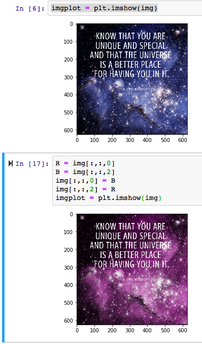
import matplotlib.pyplot as plt
import matplotlib.image as mpimg
import numpy as np

img = mpimg.imread('quote.png')
img.shape
(625, 625, 3)
Shape Manipulation
Note that the following three commands all return a modified array, but do not change the original array:- ndarray.ravel([order]) Return a contiguous flattened array. A 1-D array, containing the elements of the input, is returned.
>>> x = np.array([[1, 2, 3], [4, 5, 6]])
>>> print(np.ravel(x))
[1 2 3 4 5 6]
>>> a = np.arange(6).reshape((3, 2))
>>> a
array([[0, 1],
       [2, 3],
       [4, 5]])
>>> a = np.array([[1, 2], [3, 4]])
>>> a
array([[1, 2],
       [3, 4]])
>>> a.transpose()
array([[1, 3],
       [2, 4]])
>>> a.reshape(3,-1)
array([[ 2.,  8.,  0.,  6.],
       [ 4.,  5.,  1.,  1.],
       [ 8.,  9.,  3.,  6.]])
Stacking together different arrays
Several arrays can be stacked together along different axes:
>>> a = np.floor(10*np.random.random((2,2)))
>>> a
array([[ 8.,  8.],
       [ 0.,  0.]])
>>> b = np.floor(10*np.random.random((2,2)))
>>> b
array([[ 1.,  8.],
       [ 0.,  4.]])
>>> np.vstack((a,b))
array([[ 8.,  8.],
       [ 0.,  0.],
       [ 1.,  8.],
       [ 0.,  4.]])
>>> np.hstack((a,b))
array([[ 8.,  8.,  1.,  8.],
       [ 0.,  0.,  0.,  4.]])
>>> a = np.array((1,2,3))
>>> b = np.array((2,3,4))
>>> np.column_stack((a,b))     # with 1D arrays
array([[1, 2],
       [2, 3],
       [3, 4]])

>>> c
array([[ 8.,  8.],
       [ 0.,  0.]])
>>> d
array([[ 1.,  8.],
       [ 0.,  4.]])

>>> np.column_stack((c,d))     # with 2D arrays
array([[ 8.,  8.,  1.,  8.],
       [ 0.,  0.,  0.,  4.]])
Splitting one array into several smaller ones
- numpy.split(ary, indices_or_sections, axis=0) Split an array into multiple sub-arrays.
>>> x = np.arange(8.0)
>>> np.split(x, [3, 5, 6, 10])
[array([ 0.,  1.,  2.]),
 array([ 3.,  4.]),
 array([ 5.]),
 array([ 6.,  7.]),
 array([], dtype=float64)]
>>> a = np.floor(10*np.random.random((2,12)))
>>> a
array([[ 9.,  5.,  6.,  3.,  6.,  8.,  0.,  7.,  9.,  7.,  2.,  7.],
       [ 1.,  4.,  9.,  2.,  2.,  1.,  0.,  6.,  2.,  2.,  4.,  0.]])
>>> np.hsplit(a,3)   # Split a into 3
[array([[ 9.,  5.,  6.,  3.],
       [ 1.,  4.,  9.,  2.]]), array([[ 6.,  8.,  0.,  7.],
       [ 2.,  1.,  0.,  6.]]), array([[ 9.,  7.,  2.,  7.],
       [ 2.,  2.,  4.,  0.]])]
>>> np.hsplit(a,(3,4))   # Split a after the third and the fourth column
[array([[ 9.,  5.,  6.],
       [ 1.,  4.,  9.]]), array([[ 3.],
       [ 2.]]), array([[ 6.,  8.,  0.,  7.,  9.,  7.,  2.,  7.],
       [ 2.,  1.,  0.,  6.,  2.,  2.,  4.,  0.]])]
Copies and Views
When operating and manipulating arrays, their data is sometimes copied into a new array and sometimes not.- No Copy at All Simple assignments make no copy of array objects or of their data.
>>> a = np.arange(12)
>>> b = a            # no new object is created
>>> b is a           # a and b are two names for the same ndarray object
True
>>> b.shape = 3,4    # changes the shape of a
>>> a.shape
(3, 4)
>>> def f(x):
...     print(id(x))
...
>>> id(a)                           # id is a unique identifier of an object
148293216
>>> f(a)
148293216
>>> c = a.view()
>>> c is a
False
>>> c.base is a                        # c is a view of the data owned by a
True
>>> c.flags.owndata
False
>>>
>>> c.shape = 2,6                      # a's shape doesn't change
>>> a.shape
(3, 4)
>>> c[0,4] = 1234                      # a's data changes
>>> a
array([[   0,    1,    2,    3],
       [1234,    5,    6,    7],
       [   8,    9,   10,   11]])
>>> s = a[ : , 1:3]     # spaces added for clarity; could also be written "s = a[:,1:3]"
>>> s[:] = 10           # s[:] is a view of s. Note the difference between s=10 and s[:]=10
>>> a
array([[   0,   10,   10,    3],
       [1234,   10,   10,    7],
       [   8,   10,   10,   11]])
>>> d = a.copy()                          # a new array object with new data is created
>>> d is a
False
>>> d.base is a                           # d doesn't share anything with a
False
>>> d[0,0] = 9999
>>> a
array([[   0,   10,   10,    3],
       [1234,   10,   10,    7],
       [   8,   10,   10,   11]])
Functions and Methods Overview
- Array Creation
arange,array,copy,empty,empty_like,eye,fromfile,fromfunction,identity,linspace,logspace,mgrid,ogrid,ones,ones_like, r,zeros,zeros_like- Conversions
ndarray.astype,atleast_1d,atleast_2d,atleast_3d,mat- Manipulations
array_split,column_stack,concatenate,diagonal,dsplit,dstack,hsplit,hstack,ndarray.item,newaxis,ravel,repeat,reshape,resize,squeeze,swapaxes,take,transpose,vsplit,vstack- Questions
all,any,nonzero,where- Ordering
argmax,argmin,argsort,max,min,ptp,searchsorted,sort- Operations
choose,compress,cumprod,cumsum,inner,ndarray.fill,imag,prod,put,putmask,real,sum- Basic Statistics
cov,mean,std,var- Basic Linear Algebra
cross,dot,outer,linalg.svd,vdot
Less Basic
Broadcasting
The term broadcasting describes how numpy treats arrays with different shapes during arithmetic operations.
NumPy operations are usually done on pairs of arrays on an element-by-element basis.
>>> a = np.array([1.0, 2.0, 3.0])
>>> b = np.array([2.0, 2.0, 2.0])
>>> a * b
array([ 2.,  4.,  6.])
General Broadcasting Rules
When operating on two arrays, te dimension of 2 arrays are compatible when
- they are equal, or
- one of them is 1(scalar) Numpy can think of the scalar being stretched during the arithmetic operation, a “1” will be repeatedly prepended to the shapes of the smaller arrays until all the arrays have the same number of dimensions. Arrays with a size of 1 along a particular dimension act as if they had the size of the array with the largest shape along that dimension. The value of the array element is assumed to be the same along that dimension for the “broadcast” array.
If these conditions are not met, a ValueError: frames are not aligned exception is thrown, the size of the resulting array is the maximum size along each dimension of the input arrays.
A      (2d array):  5 x 4
B      (1d array):      1
Result (2d array):  5 x 4

A      (2d array):  5 x 4
B      (1d array):      4
Result (2d array):  5 x 4

A      (3d array):  15 x 3 x 5
B      (3d array):  15 x 1 x 5
Result (3d array):  15 x 3 x 5

A      (3d array):  15 x 3 x 5
B      (2d array):       3 x 5
Result (3d array):  15 x 3 x 5

A      (3d array):  15 x 3 x 5
B      (2d array):       3 x 1
Result (3d array):  15 x 3 x 5
>>> a = np.array([1.0, 2.0, 3.0])
>>> b = np.array([2.0, 2.0, 2.0])
>>> a * b
array([ 2.,  4.,  6.])

>>> c = 2.0
>>> a * c
array([ 2.,  4.,  6.])

>>> x = np.arange(4)
>>> x
array([0, 1, 2, 3])

>>> y = x.reshape(4,1)
>>> y
array([[0],
       [1],
       [2],
       [3]])

>>> z = np.ones(5)
>>> z
array([1., 1., 1., 1., 1.])

>>> y.shape
(4, 1)
>>> z.shape
(5,)
>>> y+z
array([[1., 1., 1., 1., 1.],
       [2., 2., 2., 2., 2.],
       [3., 3., 3., 3., 3.],
       [4., 4., 4., 4., 4.]])

>>> (y+z).shape
(4, 5)
Fancy indexing and index tricks
In addition to indexing by integers and slices, arrays can be indexed by arrays of integers and arrays of booleans.
Indexing with Arrays of Indices
>>> a = np.arange(12)**2                       # the first 12 square numbers
>>> i = np.array( [ 1,1,3,8,5 ] )              # an array of indices
>>> a[i]                                       # the elements of a at the positions i
array([ 1,  1,  9, 64, 25])
>>>
>>> j = np.array( [ [ 3, 4], [ 9, 7 ] ] )      # a bidimensional array of indices
>>> a[j]                                       # the same shape as j
array([[ 9, 16],
       [81, 49]])
Indexing with Boolean Arrays
With boolean indices , we explicitly choose which items in the array we want and which ones we don’t.
>>> a = np.arange(12).reshape(3,4)
>>> b = a > 4
>>> b                                          # b is a boolean with a's shape
array([[False, False, False, False],
       [False,  True,  True,  True],
       [ True,  True,  True,  True]])
>>> a[b]                                       # 1d array with the selected elements
array([ 5,  6,  7,  8,  9, 10, 11])

>>> a[b] = 0                                   # All elements of 'a' higher than 4 become 0
>>> a
array([[0, 1, 2, 3],
       [4, 0, 0, 0],
       [0, 0, 0, 0]])
Linear Algebra
Linear algebra (numpy.linalg)
Matrix and vector products
dot(a, b[, out]) | Dot product of two arrays. |
linalg.multi_dot(arrays) | Compute the dot product of two or more arrays in a single function call, while automatically selecting the fastest evaluation order. |
vdot(a, b) | Return the dot product of two vectors. |
inner(a, b) | Inner product of two arrays. |
outer(a, b[, out]) | Compute the outer product of two vectors. |
matmul(a, b[, out]) | Matrix product of two arrays. |
tensordot(a, b[, axes]) | Compute tensor dot product along specified axes for arrays >= 1-D. |
einsum(subscripts, *operands[, out, dtype, …]) | Evaluates the Einstein summation convention on the operands. |
einsum_path(subscripts, *operands[, optimize]) | Evaluates the lowest cost contraction order for an einsum expression by considering the creation of intermediate arrays. |
linalg.matrix_power(a, n) | Raise a square matrix to the (integer) power n. |
kron(a, b) | Kronecker product of two arrays. |
Decompositions
linalg.cholesky(a) | Cholesky decomposition. |
linalg.qr(a[, mode]) | Compute the qr factorization of a matrix. |
linalg.svd(a[, full_matrices, compute_uv]) | Singular Value Decomposition. |
Matrix eigenvalues
linalg.eig(a) | Compute the eigenvalues and right eigenvectors of a square array. |
linalg.eigh(a[, UPLO]) | Return the eigenvalues and eigenvectors of a Hermitian or symmetric matrix. |
linalg.eigvals(a) | Compute the eigenvalues of a general matrix. |
linalg.eigvalsh(a[, UPLO]) | Compute the eigenvalues of a Hermitian or real symmetric matrix. |
Norms and other numbers
linalg.norm(x[, ord, axis, keepdims]) | Matrix or vector norm. |
linalg.cond(x[, p]) | Compute the condition number of a matrix. |
linalg.det(a) | Compute the determinant of an array. |
linalg.matrix_rank(M[, tol, hermitian]) | Return matrix rank of array using SVD method |
linalg.slogdet(a) | Compute the sign and (natural) logarithm of the determinant of an array. |
trace(a[, offset, axis1, axis2, dtype, out]) | Return the sum along diagonals of the array. |
Solving equations and inverting matrices
linalg.solve(a, b) | Solve a linear matrix equation, or system of linear scalar equations. a X = b |
linalg.tensorsolve(a, b[, axes]) | Solve the tensor equation a x = b for x. |
linalg.lstsq(a, b[, rcond]) | Return the least-squares linear matrix equation ax = b. solution to a linear matrix equation. |
linalg.inv(a) | Compute the (multiplicative) inverse of a matrix. |
linalg.pinv(a[, rcond]) | Compute the (Moore-Penrose) pseudo-inverse of a matrix. |
linalg.tensorinv(a[, ind]) | Compute the ‘inverse’ of an N-dimensional array. |
Exceptions
linalg.LinAlgError | Generic Python-exception-derived object raised by linalg functions. |
>>> import numpy as np
>>> a = np.array([[1.0, 2.0], [3.0, 4.0]])
>>> print(a)
[[ 1.  2.]
 [ 3.  4.]]

>>> a.transpose()
array([[ 1.,  3.],
       [ 2.,  4.]])

>>> np.linalg.inv(a)
array([[-2. ,  1. ],
       [ 1.5, -0.5]])

>>> u = np.eye(2) # unit 2x2 matrix; "eye" represents "I"
>>> u
array([[ 1.,  0.],
       [ 0.,  1.]])
>>> j = np.array([[0.0, -1.0], [1.0, 0.0]])

>>> j @ j        # matrix product
array([[-1.,  0.],
       [ 0., -1.]])

>>> np.trace(u)  # trace
2.0

>>> y = np.array([[5.], [7.]])
>>> np.linalg.solve(a, y)
array([[-3.],
       [ 4.]])

>>> np.linalg.eig(j)
(array([ 0.+1.j,  0.-1.j]), array([[ 0.70710678+0.j        ,  0.70710678-0.j        ],
       [ 0.00000000-0.70710678j,  0.00000000+0.70710678j]]))
NPY format
The .npy format is the standard binary file format in NumPy for saving numpy arrays to disk with the full information about them.
The format stores all of the shape and dtype information necessary to reconstruct the array correctly
- .npy persisting a single arbitrary NumPy array
- .npz persisting multiple NumPy arrays on disk. ( A .npz file is a zip file containing multiple .npy files, one for each array. )

留言