Your First Machine Learning Project in Python Step-By-Step

Downloading, Installing and Starting Python SciPy

SciPy (pronounced “Sigh Pie”) is a Python-based ecosystem of open-source software for mathematics, science, and engineering. In particular, these are some of the core packages

• NumPy
Base N-dimensional array package
• SciPy library
Fundamental library for scientific computing
• Matplotlib
Comprehensive 2D Plotting
• IPython
Enhanced Interactive Console
• Sympy
Symbolic mathematics
• pandas
Data structures and analysis

The ways of installation:

• Pip

python -m pip install --user numpy scipy matplotlib ipython jupyter pandas sympy nose

The flag --user installs packages for the local user and does not write to the system directories.
• Install System-wide via a Package Manager

sudo apt-get install python-numpy python-scipy python-matplotlib ipython ipython-notebook python-pandas python-sympy python-nose

Check versions of libraries:

# Python version
import sys

print('Python: {}'.format(sys.version))
# scipy
import scipy
print('scipy: {}'.format(scipy.__version__))
# numpy
import numpy
print('numpy: {}'.format(numpy.__version__))
# matplotlib
import matplotlib
print('matplotlib: {}'.format(matplotlib.__version__))
# pandas
import pandas
print('pandas: {}'.format(pandas.__version__))
# scikit-learn
import sklearn
print('sklearn: {}'.format(sklearn.__version__))

Define Problem.

Prepare Data.

dataset

We are going to use the iris flowers dataset.

• 150 observations of iris flowers.
• 3 classes of 50 instances each
All observed flowers belong to one of 3 species: Iris Setosa, Iris Versicolour, Iris Virginica
• Attribute Information
1. sepal length in cm
2. sepal width in cm
3. petal length in cm
4. petal width in cm
5. class
For ex,, the 35th sample should be:

4.9,3.1,1.5,0.2,"Iris-setosa"

Load the dataset

• Import libraries

import pandas
from pandas.plotting import scatter_matrix
import matplotlib.pyplot as plt
from sklearn import model_selection
from sklearn.metrics import classification_report
from sklearn.metrics import confusion_matrix
from sklearn.metrics import accuracy_score
from sklearn.linear_model import LogisticRegression
from sklearn.tree import DecisionTreeClassifier
from sklearn.neighbors import KNeighborsClassifier
from sklearn.discriminant_analysis import LinearDiscriminantAnalysis
from sklearn.naive_bayes import GaussianNB
from sklearn.svm import SVC

• Load the Dataset

url = "https://raw.githubusercontent.com/jbrownlee/Datasets/master/iris.csv"
names = ['sepal-length', 'sepal-width', 'petal-length', 'petal-width', 'class']
dataset = pandas.read_csv(url, names=names)

pandas.read_csv() reads a comma-separated values (csv) file into DataFrame. names assigns a list of column names to use.
• Investigate the Dataset
• Dimensions of Dataset
How many instances (rows) and how many attributes (columns) the data contains:

# shape
print(dataset.shape)

(150, 5) means 150 instances and each with 5 attributes.
• Look at the first 20 rows of data

# head
print(dataset.head(20))

• summarize all numeric columns

# descriptions
print(dataset.describe())

• distribution of class

# class distribution
print(dataset.groupby('class').size())

• Data Visualization

The plot method on Panda's Series and DataFrame is just a simple wrapper around matplotlib.pyplot.plot().
On DataFrame, plot() is a convenience to plot all of the columns with labels.

• the distribution of the input attributes

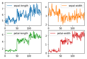
dataset.plot( subplots=True, layout=(2,2), sharex=False, sharey=False)
plt.show()


• the histogram of each input variable

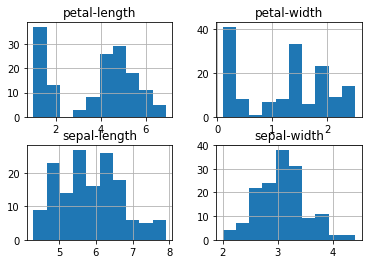
dataset.hist()
plt.show()


• the interactions between the attributes

scatter_matrix(dataset)
plt.show()

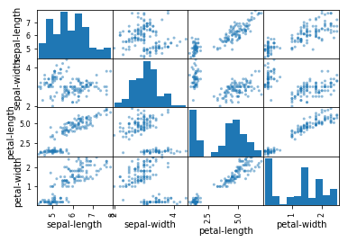Note the diagonal grouping of some pairs of attributes. This suggests a high correlation and a predictable relationship.

Create a Validation Dataset

We will split the loaded dataset into two, 80% of which we will use to train our models and 20% that we will hold back as a validation dataset.

# retrieve the numpy array
array = dataset.values
# X is the input
X = array[:,0:3]
# Y is the label
Y = array[:,4]
validation_size = 0.20
seed = 7
X_train, X_validation, Y_train, Y_validation = model_selection.train_test_split(X, Y, test_size=validation_size, random_state=seed)

• test_size : float, int or None, optional (default=None)
If float, should be between 0.0 and 1.0 and represent the proportion of the dataset to include in the test split. If int, represents the absolute number of test samples. If None, the value is set to the complement of the train size. If train_size is also None, it will be set to 0.25.

Examples of train_test_split:

>>> import numpy as np
>>> from sklearn.model_selection import train_test_split
>>> X, y = np.arange(10).reshape((5, 2)), range(5)
>>> X
array([[0, 1],
       [2, 3],
       [4, 5],
       [6, 7],
       [8, 9]])
>>> list(y)
[0, 1, 2, 3, 4]

>>> X_train, X_test, y_train, y_test = train_test_split( X, y, test_size=0.33, random_state=42)
>>> X_train
array([[4, 5],
       [0, 1],
       [6, 7]])
>>> y_train
[2, 0, 3]
>>> X_test
array([[2, 3],
       [8, 9]])
>>> y_test
[1, 4]

Now, we have training data in the X_train and Y_train for training models and validation data X_validation and Y_validation sets for validating the trained model.

Evaluate Algorithms.

We will split the dataset into 10 parts, train on 9 and test on 1 and repeat for all combinations of train-test splits.
We reset the random number seed before each run to ensure that the evaluation of each algorithm is performed using exactly the same data splits. It ensures the results are directly comparable.

seed = 7

Build Models

Let’s evaluate 6 different algorithms:

• Logistic Regression (LR)
• Linear Discriminant Analysis (LDA)
• K-Nearest Neighbors (KNN).
• Classification and Regression Trees (CART).
• Gaussian Naive Bayes (NB).
• Support Vector Machines (SVM).

Let’s build and evaluate our models:

models = []
models.append(('LR', LogisticRegression(solver='liblinear', multi_class='ovr')))
models.append(('LDA', LinearDiscriminantAnalysis()))
models.append(('KNN', KNeighborsClassifier()))
models.append(('CART', DecisionTreeClassifier()))
models.append(('NB', GaussianNB()))
models.append(('SVM', SVC(gamma='auto')))
# evaluate each model in turn
results = []
names = []
for name, model in models:
    kfold = model_selection.KFold(n_splits=10, random_state=seed)
    cv_results = model_selection.cross_val_score(model, X_train, Y_train, cv=kfold, scoring=scoring)
    results.append(cv_results)
    names.append(name)
    msg = "%s: %f (%f)" % (name, cv_results.mean(), cv_results.std())
    print(msg)

Improve Results.

Present Results.