Deep Learning with Python : A Hands-on Introduction
Deep Learning
with Python:
A Hands-on Introduction
byNikhil Ketkar
2 Machine Learning Fundamentals
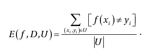
Binary Classification
Consider an abstract problem :
- We have the input and output dataset D: x --> y
- We have only a subset of this dataset: S
- Our task is to generate a computational procedure that implements the function f(x) = y for each (x,y) in S.
- We can use f to make predictions over unseen dataset U which is not in S.
- The performance of this task can be measured by mean square error
Regression
If y is a real value, this is called the regression problem.
We measure performance over this task as the root mean squared error (RMSE) over unseen data,

Consider a toy dataset:
- Inputs x are 100 values equidistantly between -1 and 1
- Observed outputs y are generated using y = 2 + x + 2 * x*x + ε ε is noise (random variation) with a normal distribution with mean 0 and the standard deviation 0.1.
- the first 80 data points as seen data and the rest as unseen data.
import numpy
import matplotlib.pyplot as plt

x = numpy.linspace(-1,1,100)
signal = 2 + x + 2 * x * x
noise = numpy.random.normal(0, 0.1, 100)
y = signal + noise

plt.plot(x, signal,'b');
plt.plot(x, y,'g')
plt.plot(x, noise, 'r')
plt.xlabel("x")
plt.ylabel("y")
plt.legend(["Without Noise", "With Noise", "Noise"], loc = 2)
plt.title('dataset')
plt.show()

To derive the matrix of the prediction model:
y = w0 + w1*x + w2*(x*x)


                     1
    = [ w0 w1 w2] [  x   ]
                   (x*x)

        y0
        y1
  Y = [ . ]
        .
        yn

           1  x0  (x0*x0)
           1  x1  (x1*x1)     w0
    = [       .           ] [ w1 ]
              .               w2
           1  xn  (xn*xn)


    = dot( X, W)

# Non-square matrices (m-by-n matrices for which m ≠ n) do not have an inverse.

  dot( transpose(X), Y ) = dot( transpose(X), dot( X, W) )
                         = dot( dot(transpose(X),X), W )

        W0
  W = [ w1 ]
        w2

   = dot(  inverse( dot(transpose(X),X) ),  dot( transpose(X), Y ))

# example to calculate the inverse of a square matrix

x = np.array([[1,2],[3,4]])
print(x)
y = np.linalg.inv(x)
print(y)
print(np.dot(x,y))

[[1 2]
 [3 4]]
[[-2.   1. ]
 [ 1.5 -0.5]]
[[1.00000000e+00 1.11022302e-16]
 [0.00000000e+00 1.00000000e+00]]
Train the polynomial model W with degree from 0 to 10:
x_train = x[0:80]
y_train = y[0:80]

# Setting sharex or sharey to True enables global sharing across the whole grid
#fig, axs = plt.subplots(10, sharex=True, sharey=False)


for degree in range(0,10):
    plt.figure()
    figtitle = "Polynomial with degree=%s" % (degree)
    plt.title(figtitle)
    plt.xlabel("x")
    plt.ylabel("y")
    x_train_power = numpy.column_stack( [numpy.power(x_train,i) for i in range(0,degree+1)] )
    A = numpy.linalg.inv( numpy.dot(x_train_power.transpose(),x_train_power) )
    B = numpy.dot( x_train_power.transpose(), y_train )
    model = numpy.dot( A , B )
    predicted = numpy.dot(model, [numpy.power(x,i) for i in range(0,degree+1)])
    plt.plot(x,y,'g')
    plt.plot(x, predicted,'r')
    plt.legend(["Actual", "Predicted"], loc = "upper left")
    train_rmse1 = numpy.sqrt(numpy.sum(numpy.dot(y[0:80] - predicted[0:80], y_train - predicted[0:80])))
    test_rmse1 = numpy.sqrt(numpy.sum(numpy.dot(y[80:] - predicted[80:], y[80:] - predicted[80:])))
    print("Train RMSE (Degree =", degree, ")", train_rmse1)
    print("Test RMSE (Degree =", degree,")", test_rmse1)
    print(model)
    plt.show()
|  |
|  |
|  |
|  |
|  |
|  |
|  |
|  |
|  |
|  |
- The RMSE of the test dataset is minimized when degree=2. W = [2.02625045 1.01902081 1.96820162]
- The RMSE of the train dataset is minimized when degree=9. W = [ 2.03631828 0.90042238 2.51542746 1.58305393 -6.91584564 -8.33112949 17.83965102 18.95676124 -8.77531865 -9.35993431]
The result shows that a higher degree model will end up just fitting the noise in addition to the signal in the data.
In the real world, we don’t know the underlying mechanism by which the data is generated.
This leads us to the fundamental challenge in machine learning, which is, does the model truly generalize?
Regularization
The model will have a low accuracy if it is overfitting. This happens because your model is trying too hard to capture the noise in your training dataset.
In a simple relation for linear regression,
y ≈ β0 + β1*x1 + β2*x2 + …+ βp*xpwhere
- Y represents the learned relation
- β represents the coefficient estimates for different variables or predictors(X)
        y1
  Y = [ y2 ]
        .
        yn


        β10 β11 ... β1p      1
    = [ β20 β21 ... β2p ] [ x1 ]
                ...         .
        βn0 βn1 ... βnp     xp

    = dot(β, X)


  loss = dot( (T - Y) , transpose(T - Y) )
The fitting procedure is to find the coefficients that they minimize this loss function.
The word regularize means to make things regular or acceptable.
Regularization discourages learning a more complex or flexible model, so as to avoid the risk of overfitting.
A regularized version for the loss function:
loss = dot( (T - Y) , transpose(T - Y) ) - λ * dot(β, transpose(β))λ is a user-defined parameter penalizing complex models.

留言