INTRODUCTION TO ALGORITHMS
Algorithms
Mastering Algorithms with C
by
Kyle Loudon
8 . Hash Tables
When a hash function can guarantee that no two keys will generate the same hash coding, the resulting hash table is said to be directly addressed. The direct addressing is rarely possible in practice.
Typically, the number of entries in a hash table is small relative to the universe of possible keys. When two keys map to the same position, they collide. A good hash function minimizes collisions, but we must still be prepared to deal with them.
Selecting a Hash Function
A hash function should distribute a set of keys about a hash table in a uniform and random manner.
A hash function h is a function we define to map a key k to some position x in a hash table. x is called the hash coding of k.
h(k) = xWhen k is not an integer, we can usually coerce it into one without much difficulty.
An example performs particularly well for strings:
- It coerces a key into a permuted integer through a series of bit operations.
- The resulting integer is mapped using the division method.
unsigned int hashpjw(const void *key) {
  const char *ptr;
  unsigned int val;

  /*****************************************************************************
  * Hash the key by performing a number of bit operations on it.
  *****************************************************************************/
  val=0;
  ptr = key;
  while (*ptr != '\0') {
    unsigned int tmp;
    val = (val << 4) + (*ptr);
    if (tmp = (val & 0xf0000000)) {
      val = val^(tmp>>24);
      val = val^tmp;
    }
    ptr++;
  }

  /*****************************************************************************
  * In practice, replace PRIME_TBLSIZ with the actual table size.
  *****************************************************************************/
  return val % PRIME_TBLSIZ;
}
Chained Hash Tables
A chained hash table fundamentally consists of an array of linked lists. Each list forms a bucket with a bucket number which is got by hashing the key.
Implementation:
- chtbl.h
#include <stdlib.h>
#include "list.h"
/*****************************************************************************
* Define a structure for chained hash tables.
*****************************************************************************/
typedef struct CHTbl_ {
  int buckets;  // the number of the array of lists
  int (*h)(const void *key);
  int (*match)(const void *key1, const void *key2);
  void (*destroy)(void *data);
  int size; // currently used number of lists
  List *lists;
} CHTbl;

/*****************************************************************************
*
*
* --------------------------- Public Interface --------------------------- *
*
*
*****************************************************************************/
int chtbl_init(CHTbl *htbl, int buckets, int (*h)(const void *key), int (*match)(const void *key1, const void *key2), void (*destroy)(void *data));
void chtbl_destroy(CHTbl *htbl);
int chtbl_insert(CHTbl *htbl, const void *data);
int chtbl_remove(CHTbl *htbl, void **data);
int chtbl_lookup(const CHTbl *htbl, void **data);

#define chtbl_size(htbl) ((htbl)->size)
#include <stdlib.h>
#include <string.h>
#include "list.h"
#include "chtbl.h"

int chtbl_init(CHTbl *htbl, int buckets, int (*h)(const void *key), int (*match)(const void *key1, const void *key2), void (*destroy)(void*data)) {
  int i;

  if ((htbl->lists = (List *)malloc(buckets * sizeof(List))) == NULL)
    return -1;

  htbl->buckets = buckets;
  for (i = 0; i < htbl->buckets; i++)
    list_init(&htbl->lists[i], destroy);

  /*****************************************************************************
  * Encapsulate the functions.
  *****************************************************************************/
  htbl->h = h;
  htbl->match = match;
  htbl->destroy = destroy;

  /*****************************************************************************
  * Initialize the number of elements in the table.
  *****************************************************************************/
  htbl->size = 0;
  return 0;
}

void chtbl_destroy(CHTbl *htbl) {
  int i;

  /*****************************************************************************
  * Destroy each bucket.
  *****************************************************************************/
  for (i = 0; i < htbl->buckets; i++) {
    list_destroy(&htbl->lists[i]);
  }

  /*****************************************************************************
  * Free the storage allocated for each list.
  *****************************************************************************/
  free(htbl->lists);

  /*****************************************************************************
  * No operations are allowed now, but clear the structure as a precaution.
  *****************************************************************************/
  memset(htbl, 0, sizeof(CHTbl));
  return;
}

int chtbl_insert(CHTbl *htbl, const void *data) {
  void *temp;
  int bucket, retval;

  /*****************************************************************************
  * Do nothing if the data is already in the table.
  *****************************************************************************/
  temp = (void *)data;
  if (chtbl_lookup(htbl, &temp) == 0)
    return 1;

  /*****************************************************************************
  * Hash the key.
  *****************************************************************************/
  bucket = htbl->h(data) % htbl->buckets;

  /*****************************************************************************
  * Insert the data into the bucket.
  *****************************************************************************/
  if ((retval = list_ins_next(&htbl->lists[bucket], NULL, data)) == 0)
    htbl->size++;
  return retval;
}

int chtbl_remove(CHTbl *htbl, void **data) {
  ListElmt *element, *prev;
  int bucket;

  /*****************************************************************************
  * Hash the key.
  *****************************************************************************/
  bucket = htbl->h(*data) % htbl->buckets;

  /*****************************************************************************
  * Search for the data in the bucket.
  *****************************************************************************/
  prev = NULL;
  for (element = list_head(&htbl->lists[bucket]); element != NULL; element =list_next(element)) {
    if ( htbl->match(*data, list_data(element)) ) {
      /***********************************************************************
      * Remove the data from the bucket.
      ***********************************************************************/
      if (list_rem _next(&htbl->lists[bucket], prev, data) == 0) {
        htbl->size--;
        return 0;
      } else {
        return -1;
      }
    }
    prev = element;
  }
  return -1;
}

int chtbl_lookup(const CHTbl *htbl, void **data) {
  ListElmt *element;
  int bucket;

  /*****************************************************************************
  * Hash the key.
  *****************************************************************************/
  bucket = htbl->h(*data) % htbl->buckets;

  /*****************************************************************************
  * Search for the data in the bucket.
  *****************************************************************************/
  for ( element = list_head(&htbl->lists[bucket]); element != NULL; element = list_next(element) ) {
    if (htbl->match(*data, list_data(element))) {
      /***********************************************************************
      * Pass back the data from the table.
      ***********************************************************************/
      *data = list_data(element);
      return 0;
    }
  }
  return -1;
}
An important application of hash tables is the way compilers maintain information about symbols encountered in a program.Compilers make use of a data structure called a symbol table. Symbol tables are often implemented as hash tables because a compiler must be able to store and retrieve information about symbols very quickly.
Open-Addressed Hash Tables
Data Structures and Algorithm Analysis in C, Second Edition
by Mark Allen WeissCHAPTER 3: LISTS, STACKS, AND QUEUES
3.1. Abstract Data Types (ADTs)
An abstract data type ( ADT ) is a set of operations. Abstract data types are mathematical abstractions. Objects such as integers, reals, and booleans have operations associated with them, and so do abstract data types.
3.2. The List ADT
A general list is of the form: a1 , a2 , a3 , . . . , an .
As a general list is considered, some popular operations are:
- print_list
- find
- insert
- delete
3.2.1. Simple Array Implementation of Lists
Obviously all of these instructions can be implemented just by using an array.
Because the running time for insertions and deletions is so slow ( O(n) for inserting at position 0 or deleting the first element ) and the list size must be known in advance, simple arrays are generally not used to implement lists.
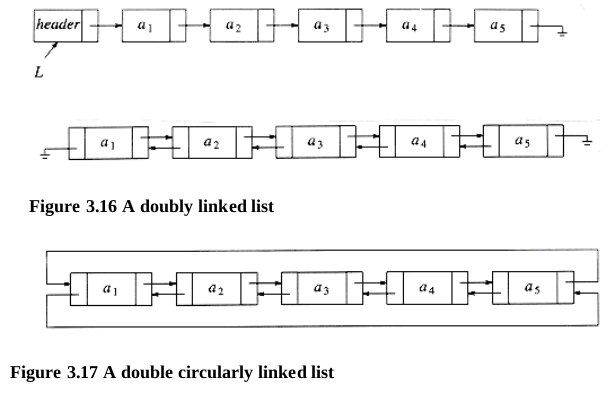
3.2.2. Linked Lists
In order to avoid the linear cost of insertion and deletion seen using array, we need to ensure that the list is not stored contiguously. The linked list consists of a series of structures, which are not necessarily adjacent in memory.
3.2.5. Doubly Linked Lists
3.2.6. Circularly Linked Lists
3.3. The Stack ADT
3.3.1. Stack Model
A stack is a list with the restriction that inserts and deletes can be performed in only one position, namely the end of the list called the top.The fundamental operations on a stack are
- push this is equivalent to an insert
- pop this deletes the most recently inserted element.
- top examine the most recently inserted element
3.3.2. Implementation of Stacks
- Linked List Implementation of Stacks The drawback of this implementation is that the calls to malloc() and free() are expensive.
- Array Implementation of Stacks We need to declare an array size ahead of time. Associated with each stack is the index for the top of stack, tos, which is -1 for an empty stack.
- To push some element x onto the stack, we increment tos and then set STACK[tos] = x
- To pop, we set the return value to STACK[tos] and then decrement tos.
struct stack_record
{
unsigned int stack_size;
int top_of_stack;
element_type *stack_array;
};
typedef struct stack_record *STACK;
#define EMPTY_TOS (-1) /* Signifies an empty stack */
3.4. The Queue ADT
Like stacks, queues are lists. With a queue, however, insertion is done at one end, whereas deletion is performed at the other end.
3.4.1. Queue Model
The basic operations on a queue are:
- enqueue This inserts an element at the end of the list (called the rear)
- dequeue it deletes (and returns) the element at the start of the list (known as the front).
3.4.2. Array Implementation of Queues
The queue data structure uses- an array, QUEUE[]
- positions q_front and q_rear, which represent the ends of the queue. Initially both 'q_front' and 'q_rear' are set to -1.
- the number of elements that are actually in the queue, q_size.
- To enqueue an element x
- Check whether queue is FULL. (q_rear == q_size-1)
- If it is FULL, then display "Queue is FULL!!! Insertion is not possible!!!" and terminate the function.
- If it is NOT FULL, then increment q_rear value by one and set QUEUE[q_rear] = x.
- To dequeue an element
- Check whether queue is EMPTY. (front == rear)
- If it is EMPTY, then display "Queue is EMPTY!!! Deletion is not possible!!!" and terminate the function.
- If it is NOT EMPTY, then increment the q_front value by one . Then display QUEUE[q_front] as deleted element. Then check whether both q_front and q_rear are equal (front == rear), if it TRUE, then set both q_front and q_rear to '-1' (front = rear = -1).
CHAPTER 4: TREES
For large amounts of input, the linear access time of linked lists is prohibitive.4.1. Preliminaries
A tree is a collection of nodes. Each node may have an arbitrary number of children. Nodes with no children are known as leaves. Nodes with the same parent are siblings. The length of a path is the number of edges on the path. For any node ni,- the depth of ni is the length of the unique path from the root to ni. Thus, the root is at depth 0.
- the height of ni is the longest path from ni to a leaf. Thus all leaves are at height 0. Thus all leaves are at height 0. The height of a tree is equal to the height of the root.
4.1.1. Implementation of Trees
If the number of children node is not fixed, keep the children of each node in a linked list of tree nodes.
typedef struct tree_node *tree_ptr;

struct tree_node
{
  element_type element;
  tree_ptr first_child;
  tree_ptr next_sibling;
};
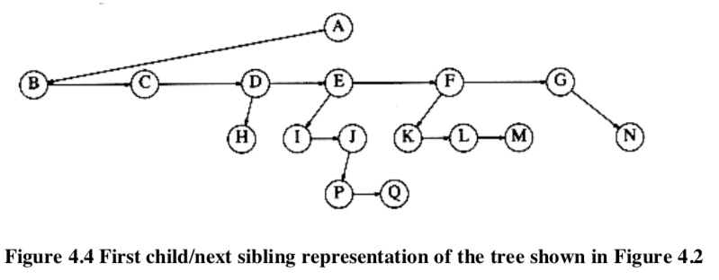 In the above tree , node E has both a pointer to a sibling (F) and a pointer to a child (I).
 4.1.2. Tree Traversals with an Application
4.2. Binary Trees
A binary tree is a tree in which no node can have more than two children.4.2.1. Implementation
typedef struct tree_node *tree_ptr;
struct tree_node
{
  element_type element;
  tree_ptr left; tree_ptr right;
};
typedef tree_ptr TREE;
4.2.2. Expression Trees
The leaves of an expression tree are operands, such as constants or variable names, and the other nodes contain operators.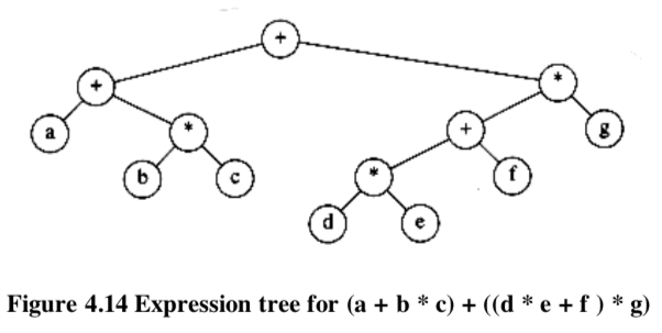
4.3. The Search Tree ADT - Binary Search Trees(BST)
An important application of binary trees is their use in searching. Let us assume that each node in the tree is assigned a key value. The property that makes a binary tree into a binary search tree is that for every node, X, in the tree,- the values of all the keys in the left subtree < the key value in X
- the values of all the keys in the right subtree > the key value in X
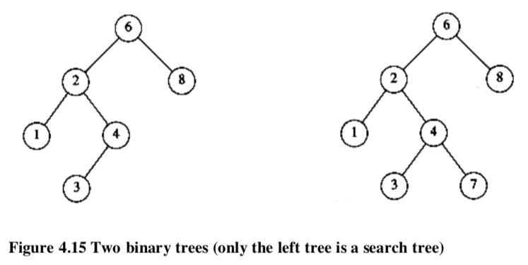 In the right of the above, there is a conflict for the node with key 7 in the left subtree of a node with key 6 .
 - Find
tree_ptr
find( element_type x, SEARCH_TREE T )
{
  if( T == NULL )
    return NULL;
  if( x < T->element )
    return( find( x, T->left ) );
  else
    if( x > T->element )
      return( find( x, T->right ) );
    else
      return T;
}
tree_ptr
insert( element_type x, SEARCH_TREE T )
{
  if( T == NULL ) {
    /* Create and return a one-node tree */
    T = (SEARCH_TREE) malloc ( sizeof (struct tree_node) );
    if( T == NULL )
      fatal_error("Out of space!!!");
    else {
      T->element = x;
      T->left = T->right = NULL;
    }
  } else
    if( x < T->element )
      T->left = insert( x, T->left );
    else
      if( x > T->element )
        T->right = insert( x, T->right );

  /* else x is in the tree already. We'll do nothing *//*11*/
  return T; /* Don't forget this line!! */
}
- If the node is a leaf it can be deleted immediately.
- If the node has one child the node can be deleted after its parent changes the child to the child of that node.
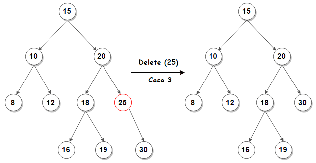
- If the node with two children
5 Hash Table
5.1. General Idea
The ideal hash table data structure is merely an array of some fixed size, containing the key objects. Typically, a key is a string. Assume the table size is H_SIZE, each key is mapped into some number in the range 0 to H_SIZE - 1 and associated object placed in the indexed cell. The mapping is called a hash function. Since there are a finite number of cells and a virtually inexhaustible supply of keys, we seek a hash function that distributes the keys evenly among the cells, deciding what to do when two keys hash to the same value (this is known as a collision), and deciding on the table size.5.2. Hash Function
If the input keys are integers, then simply returning key mod H_SIZE is generally a reasonable strategy. But, if the table size is 10 and the keys all end in zero, this is obviously a bad choice.- A simple hash function
INDEX hash( char *key, unsigned int H_SIZE ) {
  unsigned int hash_val = 0;

  while( *key != '\0' )
    hash_val += *key++;
  return( hash_val % H_SIZE );
}
INDEX hash( char *key, unsigned int H_SIZE )
{
  return ( ( key[0] + 27*key[1] + 729*key[2] ) % H_SIZE ); }
}
This only uses the first 3 characters as the key, the key is computed as : hk = k1 + ((k3) * 27 + k2) * 27the H_SIZE is 17,576 = 26 x 26 x 26. In real usage of English, the number of different combinations is actually only 2,851. The space is a waste.
INDEX
hash( char *key, unsigned int H_SIZE )
{
  unsigned int hash_val = O;

  while( *key != '\0' )
    hash_val = ( hash_val << 5 ) + *key++;
  return( hash_val % H_SIZE );
}
Some programmers implement their hash function by using only the characters in the odd spaces. If, when inserting an element, it hashes to the same value as an already inserted element, then we have a collision and need to resolve it. We will discuss two of the simplest strategies,: open hashing(separate chaining) and closed hashing(open addressing). 5.3. Open Hashing (Separate Chaining)
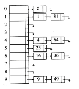
Keep a list of all elements that hash to the same value. Assume the hashing function is used for for the first 10 square numbers:hash(x) = x mod 10the hash table looks like:
 A sample implementation :
 - type declarations
typedef struct list_node * node_ptr;

struct list_node
{
  element_type element;
  node_ptr next;
};

typedef node_ptr LIST;
typedef node_ptr position;
/* LIST *the_list will be an array of lists, allocated later */
/* The lists will use headers, allocated later */
struct hash_tbl
{
  unsigned int table_size;
  LIST *the_lists;
};

typedef struct hash_tbl * HASH_TABLE;
HASH_TABLE initialize_table( unsigned int table_size )
{
  HASH_TABLE H;
  int i;

  if( table size < MIN_TABLE_SIZE ) {
    error("Table size too small");
    return NULL;
  }

  /* Allocate table */
  H = (HASH_TABLE) malloc ( sizeof (struct hash_tbl) );
  if( H == NULL )
    fatal_error("Out of space!!!");
  // sets the table size to a prime number
  H->table_size = next_prime( table_size );
  /* Allocate list pointers */
  H->the_lists = (position *) malloc( sizeof (LIST) * H->table_size );
  if( H->the_lists == NULL )
    fatal_error("Out of space!!!");

  /* Allocate list headers for each hash value,
     the header is not used to store element info
   */
  for(i=0; itable_size; i++ ) {
    H->the_lists[i] = (LIST) malloc( sizeof (struct list_node) );
    if( H->the_lists[i] == NULL )
      fatal_error("Out of space!!!");
    else
      H->the_lists[i]->next = NULL;
  }
  return H;
}
position find( element_type key, HASH_TABLE H )
{
  position p;
  LIST L;

  L = H->the_lists[ hash( key, H->table_size) ]; // header
  p = L->next;
  while( (p != NULL) && (p->element != key) )
    p = p->next;
  return p;
}
void insert( element_type key, HASH_TABLE H )
{
  position pos, new_cell;
  LIST L;

  pos = find( key, H );
  if ( pos == NULL ) {
      new_cell = (position) malloc(sizeof(struct list_node));
      if( new_cell == NULL )
        fatal_error("Out of space!!!");
      else {
        L = H->the_lists[ hash( key, H->table size ) ];// header
        L->next = new_cell;
        new_cell->next = NULL;
        new_cell->element = key; /* Probably need strcpy!! * /
      }
  }

}
Any scheme could be used besides linked lists to resolve the collisions. 5.4. Closed Hashing (Open Addressing)
In a closed hashing system, if a collision occurs, alternate cells are tried until an empty cell is found.MIT 6.006 Introduction to Algorithms, Fall 2011
- Lecture 1: Algorithmic Thinking, Peak Finding
- Lecture 2: Models of Computation, Document Distance
- Lecture 3: Insertion Sort, Merge Sort
- Lecture 4: Heaps and Heap Sort
- Lecture 5: Binary Search Trees, BST Sort
- Lecture 6: AVL Trees, AVL Sort
AVL tree is a self-balancing Binary Search Tree (BST) where the difference between heights of left and right subtrees cannot be more than one for all nodes.
Most of the BST operations (e.g., search, max, min, insert, delete.. etc) take O(h) time where h is the height of the BST. The cost of these operations may become O(n) for a skewed Binary tree.
If we make sure that height of the tree remains O(log(n)) after every insertion and deletion, then we can guarantee an upper bound of O(log(n)) for all these operations.
To make sure that the given tree remains AVL after every insertion, we must augment the standard BST insert operation to perform some re-balancing. To re-balance a BST without violating the BST property:
keys(left) < key(root) < keys(right)
balanceFactor = height(left subtree) - height(right subtree)
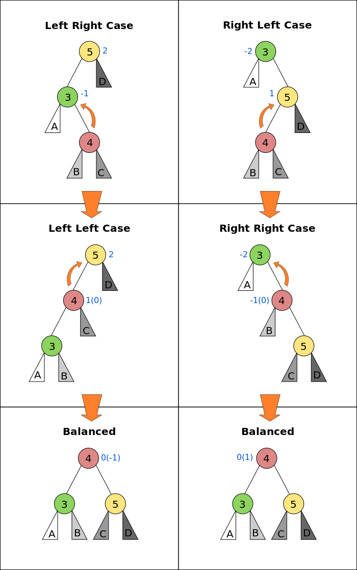 There can be 4 possible cases that needs to be rotated: T1, T2, T3 and T4 are subtrees.
 - Left Left Case
         z                                      y
        / \                                   /   \
       y   T4      Right Rotate (z)          x      z
      / \          - - - - - - - - ->      /  \    /  \
     x   T3                               T1  T2  T3  T4
    / \
  T1   T2
     z                               z                           x
    / \                            /   \                        /  \
   y   T4  Left Rotate (y)        x    T4  Right Rotate(z)    y      z
  / \      - - - - - - - - ->    /  \      - - - - - - - ->  / \    / \
T1   x                          y    T3                    T1  T2 T3  T4
    / \                        / \
  T2   T3                    T1   T2
  z                                y
 /  \                            /   \
T1   y     Left Rotate(z)       z      x
    /  \   - - - - - - - ->    / \    / \
   T2   x                     T1  T2 T3  T4
       / \
     T3  T4
   z                            z                            x
  / \                          / \                          /  \
T1   y   Right Rotate (y)    T1   x      Left Rotate(z)   z      y
    / \  - - - - - - - - ->     /  \   - - - - - - - ->  / \    / \
   x   T4                      T2   y                  T1  T2  T3  T4
  / \                              /  \
T2   T3                           T3   T4
struct node
{
int val;            //value
struct node* left;  //left child
struct node* right; //right child
int ht;             //height of the node
} node;
- Insertion


INTRODUCTION TO ALGORITHMS
by THOMAS H. CORMEN CHARLES E. LEISERSON RONALD L. RIVEST CLIFFORD STEINThe Role of Algorithms in Computing
1.1 Algorithms
An algorithm is a sequence of computational steps that transform the input into the output. The statement of the problem specifies in general terms the desired input/output relationship. The algorithm describes a specific computational procedure for achieving that input/output relationship. Sorting is a simple example algorithm.1.2 Algorithms as a technology
We should consider algorithms, like computer hard-ware, as a technology. Total system performance depends on choosing efficient algorithms as much as on choosing fast hardware.Getting Started
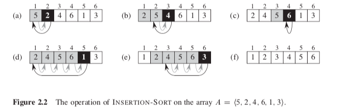
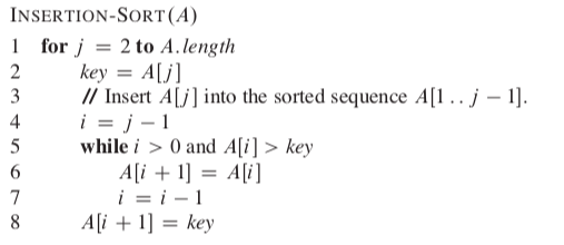
2.1 Insertion sort
The sorting problem: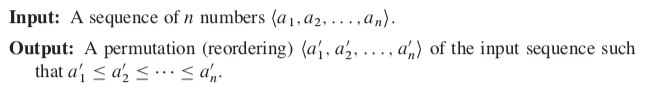
 C:
C:
#include

int main(int argc, char *argv[] ){

 char A[6] = {5, 2, 4, 6, 1, 3};
 int i=0, j=0, l=0, key=0;

 l = sizeof(A);

 for ( j=1; j -1) && (A[i] >  key) ){
   A[i+1] = A[i];
   i=i-1;
  }
  A[i+1] = key;
 }

 printf("Sorted: ");
 i = 0;
 while (i< l){
  printf("%d ", A[i]);
  i++;
 }
 printf("¥n");
}
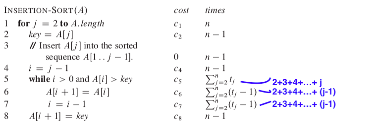
2.2 Analyzing algorithms
Analyzing an algorithm has come to mean predicting the resources that the algorithm requires:- memory
- bandwidth
- computational time
- The random-access machine (RAM) model: instructions are executed one after another, with no concurrent operations.
- Each instruction takes a constant amount of time.
T(n)Assume that each execution of the i-th line takes a constant time, the running time of the algorithm is the sum of running times for each statement executed. Different types of analysis can be done:
- worst-case running time For ex., searches for absent information.
- average-case running time Calculate computing time for all of the inputs then calculate the mean of all the computed time.
- best-case running time A minimum number of operations to be considered to be executed for a particular input. For ex., sorting for a sorted input sequence.
- Θ Notation (Theta notation)
3n³ + 40n² - 10n + 409 = Θ(n³)The constant factor don't tell us about the rate of growth of the running time. The Θ Notation follows simple two rules:
- Drop low order terms
- Ignore leading constants.
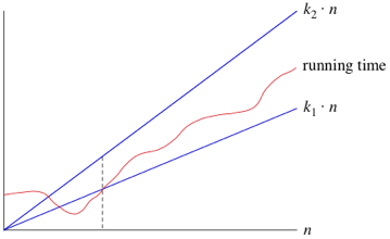 When we use Θ notation, we're saying that we have an asymptotically tight bound on the running time. "Asymptotically" because it matters for only large values of n. "Tight bound" because we've nailed the running time to within a constant factor above and below. If the time is independent of n, we write Θ(1).
 The running time:
- the best case occurs if the array is already sorted The while loop is not entered.
- the worst case occurs if the array is in reverse sorted order
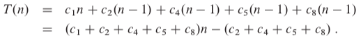 It is thus a linear function of n.
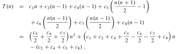 It is thus a quadratic function of n.
 2.3 Designing algorithms
Many useful algorithms are recursive in structure and typically follow a divide-and-conquer approach: they break the problem into several subproblems, subproblems are solved recursively. The merge sort algorithm closely follows the divide-and-conquer paradigm. Intuitively, it operates as follows.- Divide Divide the n-element sequence to be sorted into two subsequences of n/2 elements each.
- Conquer Sort the two subsequences recursively using merge sort.
- Combine Merge the two sorted subsequences to produce the sorted answer. This is the key operations. We merge by calling an auxiliary procedure
MERGE( A, p, q, r )where A is an array and p, q, and r are indices into the array such that p < q < r. The procedure assumes that the subarrays A[p ... q] and A[q ... r] are in sorted order. It merges them to form a single sorted subarray that replaces the current subarray A[p ... r]. The MERGE() works like:
- Compare the smallest number from 2 input arrays then move the smallest one to the final array
- Repeat the above step until one array is empty
- Append the remained array to the final array
n1 = q - p + 1
n2 = r - q
let L[1...(n1+1)] and R[1...(n2+1)] be new arrays
for i=1 to n1
    L[i] = A[p+i-1]
L[n1+1] = INF
for j=1 to n2
    R[j] = A[q+j]
R[n2+1] = INF
i = j = 1
for k=p to r
    if L[i] <= R[j]
        A[k] = L[i]
        i = i + 1
    else
        A[k] = R[j]
        j = j +1
- the first 2 loops Take Θ(n1 + n2) = Θ(n)
- the last loop There are n iterations, n = r - p + 1.
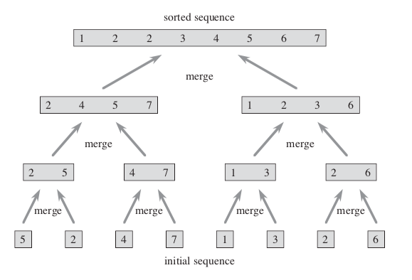
MERGE-SORT(A, p, r){
    if p < r
        q = [(p+r)/2]
        MERGE-SORT(A, p, q)
        MERGE-SORT(A, q+1, r)
        MERGE(A, p, q, r)
}
The un-sorted array { 5, 2, 4, 7, 1, 3, 2, 6 } is used to illustrate the recursive operations:
 When an algorithm contains a recursive call to itself, we can often describe its running time by recurrences, which describes the overall running time on a problem of size n in terms of the running time on smaller inputs. Suppose that
 - T(n) be the running time on a problem of size n.
- our division of the problem yields a subproblems, each of which is 1/b the size of the original. It takes time T(n/b) to solve one subproblem of size n/b, and so it takes time a*T(n/b) to solve a subproblems.
- D(n) time to divide the problem into subproblems
- C(n) time to combine the solutions to the subproblems into the solution to the original problem
T(n) = a *T(n/b) + D(n) + C(n)Use MERGE-SORT() as an example, consider the worst-case running time of merge sort on n numbers:
- Divide The divide step just computes the middle of the subarray, which takes constant time. Thus, D(n) = Θ(1)
- Conquer We recursively solve two subproblems, each of size n/2, which contributes 2*T(n/2) to the running time.
- Combine We have already noted that the MERGE procedure on an n-element subarray takes time Θ(n), and so C(n) = Θ(n)
T(n) = 2 * T(n/2) + Θ(n)Θ(n) represents the time required to divide and combine steps with the input size n. Let's use the constant c to represent Θ(1). That is, c represents the time required to solve problems of size 1.
T(n) = 2 * T(n/2) + c*n
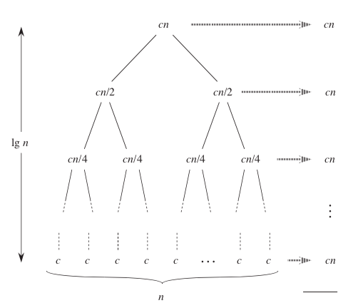 The fully expanded tree has lg(n) + 1 levels , and each level contributes a total cost of cn. The total cost, therefore, is cn*lg(n) + cn, which is Θ(n * lg(n)). Implementation in C:
#include <stdio.h>
#include <unistd.h>

void merge(int *A, int p, int q, int r){
 int n1 = q - p +1;
 int n2 = r - q;
 int L[n1], R[n2];
 int i,j,k;

 for ( i=0; i<n1; i++)
  L[i] = A[p+i];
 for ( j=0; j<n2; j++)
  R[j] = A[q+1+j];
 i =j = 0;
 for ( k=p; k<r+1; k++){
  if ( (j==n2) || ( (i<n1) && (L[i] <= R[j]) ) ) {
   A[k] = L[i];
   i++;
  } else {
   A[k] = R[j];
   j++;
  }
 }

}

void mergeSort(int *A, int p, int r){
 int q;
 printf("mergeSort:%d-%d\n", p, r);

     if (p < r) {
         q = (p+r)/2;
         mergeSort(A, p, q);
         mergeSort(A, q+1, r);
         merge(A, p, q, r);
 }
}

int main(int argc, char *argv[] ){
 int A[8]={5, 2, 4, 7, 1, 3, 2, 6 };
 int i=0;
 int len = sizeof(A)/sizeof(int);

 mergeSort(A, 0, len-1);
}
3 Growth of Functions
3.1 Asymptotic notation
For a given function g(n), a function f(n) belongs to the set Θ( g(n) ) if there exist positive constants c1 and c2 such that it can be “sandwiched” between c1*g(n) and c2*g(n), for sufficiently large n. Θ( g(n) ) is a set, we use Θ( g(n) ) = f(n) to express the same notion.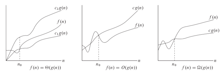 For all n >= n0, the function f(n) is equal to g(n) to within a constant factor. We say that g(n) is an asymptotically tight bound for f(n). For ex., to prove
Θ( n*n ) = (n*n)/2 - 3*n
c1 * (n*n) <= (n*n)/2 - 3*n <= c2 *(n*n)
c1 = 1/14 , c2 = 1/2, n0 = 7
0 <= f(n) <= c * g(n) , for all n >= n0
3.2 Standard notations and common functions
4 Divide-and-Conquer
4.1 The maximum-subarray problem
Consider to maximize the profit from the stock.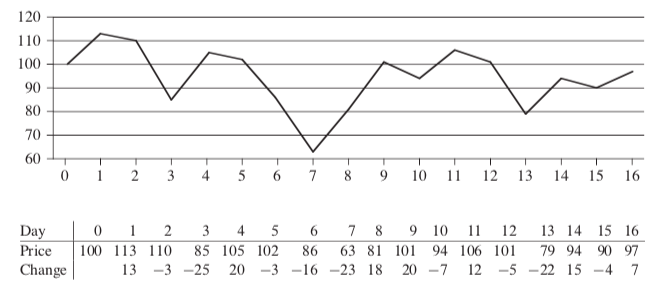 The following demonstrating that the maximum profit sometimes comes neither by buying at the lowest price nor by selling at the highest price.
 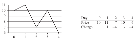 The price of $7 after day 2 is not the lowest price overall, and the price of $10 after day 3 is not the highest price overall. A brute-force solution to this problem: just try every possible pair of buy and sell dates in which the buy date precedes the sell date.
n! / ( 2! * (n-2)! ) = n * (n-1) /2
- consider the daily change in price(today - yesterday) as an array A Positive is price up, negative is price down.
- find the nonempty, contiguous subarray of A whose values have the largest sum The more the sum, the more the net profit after selling it. Call this the maximum subarray.
- entirely in the subarray A[low ... mid], so that low <= i<= j<= mid
- entirely in the subarray A[mid-1 ... high], so that mid <= i <= j <= high
- crossing the midpoint, so that low <= i <= mid < j <= high
FIND-MAX-CROSSING-SUBARRAY( A, low, mid, high) {
  left-sum = A[mid]
  sum = 0
  for i = mid-1 downto low
    sum = sum + A[i]
    if sum > left-sum
      left-sum = sum
      max-left = i
  right-sum = A[mid+1]
  sum = 0
  for j = mid+2 to high
    sum = sum + A[j]
    if sum > right-sum
      right-sum = sum
      max-right = j
  return (max-left, max-right, left-sum + right-sum)

}
FIND-MAXIMUM-SUBARRAY(A, low, high) {
  if high == low
    return (low, high, A[low]) // base case: only one element   Θ(1)
  else
    mid = [(low + high)/=2]
    (left-low, left-high, left-sum) = FIND-MAXIMUM-SUBARRAY(A, low, mid)   T(n/2)
    (right-low, right-high, right-sum) = FIND-MAXIMUM-SUBARRAY(A, mid+1, high)   T(n/2)
    (cross-low; cross-high; cross-sum = FIND-MAX-CROSSING-SUBARRAY(A, low, mid, high)  Θ(n)
    if left-sum >= right-sum and left-sum >= cross-sum
      return (left-low, left-high, left-sum)    &Theta(1)
    elseif right-sum >= left-sum and right-sum >= cross-sum
      return (right-low, right-high, right-sum)
    else
      return (cross-low, cross-high, cross-sum)
}
  T(n) = Θ(1) + 2* T(n/2) + Θ(n) + Θ(1)
       = Θ(1) + 2* T(n/2) + Θ(n)
T(n) = Θ( n* lgn )
4.2 Strassen’s algorithm for matrix multiplication
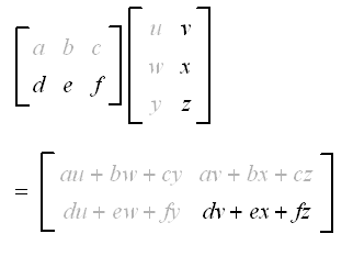
C = AB
 If A and B are n x n matrixes, the pseudo code:
SQUARE-MATRIX-MULTIPLY(A, B){
n = A:rows
let C be a new n x n matrix
for i = 1 to n
for j = 1 to n
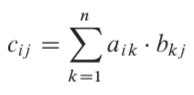
cij = 0
for k = 1 to n
cij = cij + aik * bkj
return C
}
 We can use these equations to create a straightforward, recursive, divide-and-conquer algorithm:
SQUARE-MATRIX-MULTIPLY-RECURSIVE(A, B){
n = A.rows
let C be a new n x n matrix
if n==1
c11 = a11 * b11
else
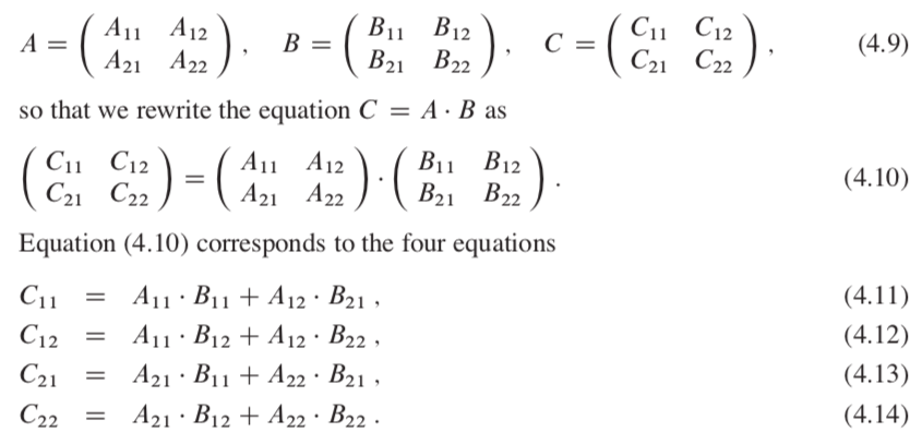
partition A, B, and C as in equations (4.9)
C11 = SQUARE-MATRIX-MULTIPLY-RECURSIVE(A11, B11) + SQUARE-MATRIX-MULTIPLY-RECURSIVE(A12, B21)
C12 = SQUARE-MATRIX-MULTIPLY-RECURSIVE(A11, B12) + SQUARE-MATRIX-MULTIPLY-RECURSIVE(A12, B22)
C21 = SQUARE-MATRIX-MULTIPLY-RECURSIVE(A21, B11) + SQUARE-MATRIX-MULTIPLY-RECURSIVE(A22, B21)
C22 = SQUARE-MATRIX-MULTIPLY-RECURSIVE(A21, B12) + SQUARE-MATRIX-MULTIPLY-RECURSIVE(A22, B22)
return C
}
T(n) = Θ(1) + 8*T(n/2) + Θ(n*n)
     =  8*T(n/2) + Θ(n*n)
4.3 The substitution method for solving recurrences
4.4 The recursion-tree method for solving recurrences
4.5 The master method for solving recurrences
4.6 Proof of the master theorem
5 Probabilistic Analysis and Randomized Algorithms
5.1 The hiring problem
5.2 Indicator random variables
5.3 Randomized algorithms
5.4 Probabilistic analysis and further uses of indicator random variables
6 Heapsort
The heapsort combines the better attributes of the two sorting algorithms:- Like insertion sort heapsort sorts in place: only a constant number of array elements are stored outside the input array at any time
- Like merge sort heapsort’s running time is O( n*lg(n) )
6.1 Heaps
The (binary) heap data structure(the key of parent >= (<=) the keys of children) is an array object that we can view as a nearly complete binary tree.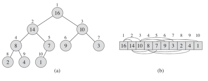 An array A that represents a heap is an object with two attributes:
 - A.length the number of elements in the array
- A.heapSize how many elements in the heap are currently stored within array A.
- PARENT(i) return (i/2)
- LEFT(i) return 2i
- RIGHT(i) return (2i + 1)
- max-heaps A[PARENT(i)] >= A[i]
- min-heaps A[PARENT(i)] <= A[i]
6.2 Maintaining the heap property
In order to maintain the max-heap property, we call the procedure MAX-HEAPIFY:
MAX-HEAPIFY(A, i){
  l = LEFT(i)
  r = RIGHT(i)
  if (l <= A.heapSize) and (A[l] > A[i])
    largest = l
  else
    largest = i
  if (r <= A.heapSize) and (A[r] > A[largest])
   largest = r
  if largest != i
    exchange A[i] with A[largest]
    MAX-HEAPIFY(A, largest)
}
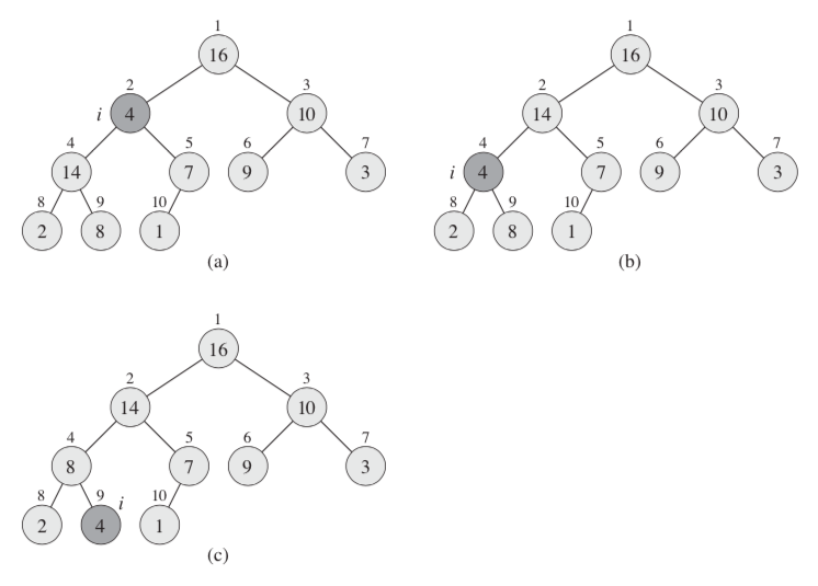 If the sub-tree node is changed, its children node may violate the max-heap property. The running time of MAX-HEAPIFY on a subtree of size n rooted at a given node i is the Θ(1) time, plus the time to run MAX-HEAPIFY on a subtree rooted at one of the children of node i . The children’s subtrees each have size at most 2n/3 — the worst case occurs when the bottom level of the tree is exactly half full. Why? Assume that the total number of nodes in the tree is n, the height of the tree is h, the worst case:
  n = 1 + 2 + 4 + ... + 2 exp(h-1)
    = [ 1- 2 exp(h) )/(1-2)
    = 2 exp(h) - 1

  n = 1 + (Number of nodes in Left Subtree) + (Number of nodes in Right Subtree)
    = 1 + [ 1+2+4+...+ 2 exp(h-2) ] + [ 1+2+4+...+ 2 exp(h-3) ]
    = 1 + [ ( 1- 2 exp(h-1) )/(1-2) ] + [ ( 1- 2 exp(h-2) )/(1-2) ]
    = 1 + [ 2 exp(h-1) - 1 ] +  [ 2 exp(h-2) - 1]
    = 2 * [ 2 exp(h-2) ] + 2 exp(h-2) - 1
    = 3 * [ 2 exp(h-2) ] - 1

  [ 2 exp(h-2) ] = (n+1)/3

  (Number of nodes in Left Subtree) = 2 exp(h-1) - 1
                                    = 2 [ 2 exp(h-2) ] -1
                                    = 2*(n+1)/3 - 1
                                    = (2*n - 1)/3
                                    < 2n/3
T(n) = T(2n/3) + Θ(1)
6.3 Building a heap
We can use the procedure MAX-HEAPIFY in a bottom-up manner. The elements in the subarray A[ (n/2 +1) ... n ] are all leaves of the tree. The procedure BUILD-MAX-HEAP:
BUILD-MAX-HEAP(A) {
  A.heapSize = A.length
  for i = (A.length/2) downto 1
    MAX-HEAPIFY(A, i)
}
6.4 The heapsort algorithm
The heapsort algorithm starts by using BUILD-MAX-HEAP to build a max-heap. Then repeat the following process:- Put the maximum element (stored at the root A[1]) into its correct final position A[n]
- Decrementing A.heapSize to discard node n from the heap
- Call MAX-HEAPIFY(A, 1) to fix the max-heap property broken by node 1.
HEAPSORT(A) {
  BUILD-MAX-HEAP(A)
  for i = A.length downto 2
    exchange A[1] with A[i]
    A.heapSize = A.heapSize - 1
    MAX-HEAPIFY(A, 1)
}
6.5 Priority queues
As with heaps, priority queues come in two forms: max-priority queues and min-priority queues. A priority queue is a data structure for maintaining a set S of elements, each with an associated value called a key. A typical priority queue supports following operations:- insert(item, priority) Inserts an item with given priority.
- getHighestPriority() Returns the highest priority item.
- deleteHighestPriority() Removes the highest priority item.
/ C code to implement Priority Queue
// using Linked List
#include <stdio.h>
#include <stdlib.h>

// Node
typedef struct node {
    int data;
    // Lower values indicate higher priority
    int priority;
    struct node* next;

} Node;

// Function to Create A New Node
Node* newNode(int d, int p)
{
    Node* temp = (Node*)malloc(sizeof(Node));
    temp->data = d;
    temp->priority = p;
    temp->next = NULL;

    return temp;
}

// Return the value at head
int peek(Node** head)
{
    return (*head)->data;
}

// Removes the element with the
// highest priority form the list
void pop(Node** head)
{
    Node* temp = *head;
    (*head) = (*head)->next;
    free(temp);
}

// Function to push according to priority
void push(Node** head, int d, int p)
{
    Node* start = (*head);

    // Create new Node
    Node* temp = newNode(d, p);

    // Special Case: The head of list has lesser
    // priority than new node. So insert new
    // node before head node and change head node.
    if ((*head)->priority < p) {
        // Insert New Node before head
        printf("insert (%d,%d) before head(%d,%d)\n", d, p, (*head)->data , (*head)->priority );
        temp->next = *head;
        (*head) = temp;
    }
    else {
        // Traverse the list and find a
        // position to insert new node
        while (start->next != NULL &&
               start->next->priority > p) {
            start = start->next;
        }

        // Either at the ends of the list
        // or at required position
        temp->next = start->next;
         printf("insert (%d,%d) after  (%d,%d)\n", d, p,  start->data, start->priority );
        start->next = temp;
    }
}

// Function to check is list is empty
int isEmpty(Node** head)
{
    return (*head) == NULL;
}

int main() {
    // Create a Priority Queue
    // 7->4->5->6
    Node* pq = newNode(4, 1);
    push(&pq, 5, 2);
    push(&pq, 6, 3);
    push(&pq, 7, 0);

    while (!isEmpty(&pq)) {
        printf("%d ", peek(&pq));
        pop(&pq);
    }

    return 0;

}
insert (5,2) before head(4,1)
insert (6,3) before head(5,2)
insert (7,0) after  (4,1)
6 5 4 7
7 Quicksort
7.1 Description of quicksort 170 7.2 Performance of quicksort 174 7.3 A randomized version of quicksort 179 7.4 Analysis of quicksort 1808 Sorting in Linear Time
8.1 Lower bounds for sorting 191 8.2 Counting sort 194 8.3 Radix sort 197 8.4 Bucket sort 2009 Medians and Order Statistics
9.1 Minimum and maximum 214 9.2 Selection in expected linear time 215 9.3 Selection in worst-case linear time 22011 Hash Tables
A hash table is an effective data structure for implementing dictionaries. When the number of keys actually stored is small relative to the total number of possible keys, hash tables become an effective alternative to directly addressing an array. Instead of using the key as an array index directly, the array index is computed from the key.11.1 Direct-address tables
We use an array, or direct-address table, denoted by T [0,..., m-1], in which each position, or slot, corresponds to a key.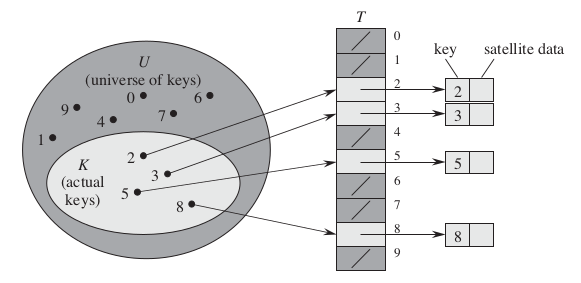
The object or a pointer of the object is stored in the table's slot . The dictionary operations are trivial to implement:
- search
DIRECT-ADDRESS-SEARCH(T, k){
 return T[k];
}
DIRECT-ADDRESS-INSERT(T, x){
  T[x.key] = x;
}
DIRECT-ADDRESS-DELETE(T, x){
  T[x.key] = NIL;
}
}
11.2 Hash tables
With direct addressing, an element with key k is stored in slot k. With hashing, this element is stored in slot h(k). The slot is computed from the key using a hash function. Here, h maps the universe U of keys into the slots of a hash table T[0 ... m-1].
h:U ---> {0, 1, ..., m-1 }
the size of the hash table m is typically much less than the size of U. h(k) is the hash value of key k. 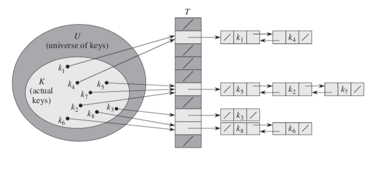 The collision happens when two more keys may hash to the same slot. Collision resolutions can be resolved by chaining:
 - All the elements hashed to the same slot are put into the same linked list.
- Slot j contains a pointer to the head of the list of all stored elements that hash to j ; if there are no such elements, slot j contains NIL .
CHAINED-HASH-INSERT(T, x){
 insert x at the head of list T[ h(x.key) ]
}

CHAINED-HASH-SEARCH(T, k){
 search for an element with key k in list T[ h(k) ]
}

CHAINED-HASH-DELETE(T, x){
 delete x from the list T[ h(x.key) ]
}
The insertion procedure is fast in part because it assumes that the element x being inserted is not already present in the table; if necessary, we can check this assumption (at additional cost) by searching for an element whose key is x:key before we insert. Given a hash table T with m slots that stores n elements, define the load factor α for T as n/mThe average-case performance of hashing depends on how well the hash function h() distributes the set of keys to be stored among the m slots, on the average.
11.3 Hash functions
To hash the key, keys are often interpreted as natural numbers. Most hash functions assume that the universe of keys is the integer space. For this, we can interpret a character string as an integer expressed in suitable radix notation. Fo ex., the string "pt" as the pair of decimal integers (112, 116), since p = 112 and t = 116 in the ASCII character set; then, we can use a radix-128 integer to represent the key "pt", it becomes:112 x 128 + 116 = 14452.
11.3.1 The division method
We map a key k into one of m slots by taking the remainder of k divided by m:h(k) = k mod mA prime not too close to an exact power of 2 is often a good choice for m.
11.3.2 The multiplication method
- define a constant A in the range 0 <<A < 1
- multiply the key k by A
- extract the fractional part in (k * A)
- multiply this value by m and take the floor
h(k) = [ m * ( (k * A ) mod 1 ) ]
11.3.3 Universal hashing
11.4 Open addressing
In open addressing, all elements occupy the hash table itself. That is, each table entry contains either an element or NIL, the hash table can “fill up” so that no further insertions can be made.12 Binary Search Trees (BST)
12.1 What is a binary search tree?
In addition to a key and satellite data, each node contains attributes left, right, and p that point to the nodes corresponding to its left child, its right child, and its parent, respectively. The binary-search-tree property: Let x be a node in a binary search tree:- If y is a node in the left subtree of x, then y.key <= x.key
- If y is a node in the right subtree of x, then y.key >= x:key
INORDER-TREE-WALK(x) {
  if (x != NIL ){
    INORDER-TREE-WALK(x.left);
    print x.key;
    INORDER-TREE-WALK(x.right);
  }
}
Similarly, a preorder tree walk prints the root before the values in either subtree, and a postorder tree walk prints the root after the values in its subtrees. 12.2 Querying a binary search tree
- Searching
TREE-SEARCH( x; k) {
  if (x == NIL) or (k==x.key)
   return x
  if (k < x.key )
    return TREE-SEARCH(x.left; k)
  else
    return TREE-SEARCH(x.right; k)
}
TREE-MINIMUM(x) {
  while ( x.left != NIL )
    x = x.left
  return x
}
TREE-MAXIMUM(x) {
  while (x.right != NIL)
    x = x:right
  return x
}
TREE-SUCCESSOR (x) {
  # case 1
  if ( x.right != NIL )
    return TREE-MINIMUM(x.right)
  # case 2
  y = x.p
  while ( y != NIL ) and ( x == y.right ) {
    x = y
    y = y.p
  }
 return y
}
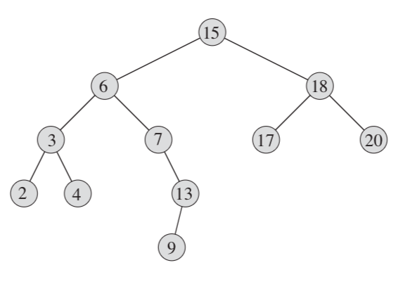
- case 1: If the right subtree of node x is nonempty, just find the minimum from the right subtree . The successor of the node with key 15 in the above figure is the node with key 17.
- case 2: If the right subtree of node x is empty, then y is the lowest ancestor of x whose left child is also an ancestor of x. the successor of the node with key 13 is the node with key 15.
12.3 Insertion and deletion
- Insertion
TREE-INSERT (T, z){
  y = NIL;
  x = T.root
  // find the parent
  while (x != NIL) {
    y = x;
    if  ́(z.key < x.key)
      x = x.left;
    else
      x = x.right
  z.p = y;
  if (y == NIL)
    T.root = z //tree T was empty
  else if  (z.key < y:key)
    y.left = z
  else
    y.right = z
}
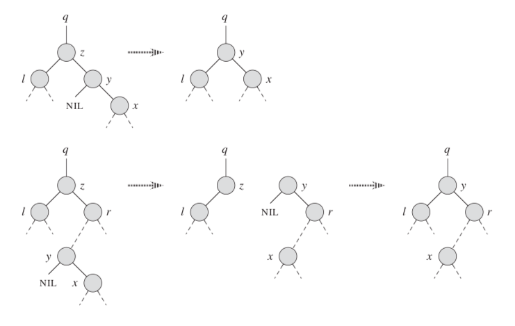
- If z has no children we simply remove it by modifying its parent to replace z with NIL as its child.
- If z has just one child we elevate that child to take z's position in the tree by modifying z's parent to replace z by z'ss child.
- If z has two children we find z's successor y which must be in z's right subtree, and have y take z's position in the tree. The rest of z's original right subtree becomes y’s new right subtree, and z's left subtree becomes y’s new left subtree. In order to move subtrees around within the binary search tree, we define a subroutine TRANSPLANT() , which replaces one subtree as a child of its parent with another subtree.
TRANSPLANT (T, u, v) {
  if ( u.p == NIL )
    T.root = v
  else if ( u == u.p.left ) // us is the left child of p
    u.p.left = v
  else
    u.p.right = v

  if ( v != NULL)
    v.p = u.p
}
With the T RANSPLANT procedure in hand, to delete a noze z from T:
TREE-DELETE (T, z): {
  if (z.left == NIL)
    TRANSPLANT(T, z, z.right);
  else if (z.right == NIL)
    TRANSPLANT(T, z, z.left);
  else
    y = TREE-MINIMUM (z.right);
    if (y.p != z) {
      TRANSPLANT (T, y, y.right);
      y.right = z.right;
      y.right.p = y;
    TRANSPLANT (T, z, y);
    // y has no left child
    y.left = z.left
    y.left.p = y
}

留言