Wavelet Transform
The Wavelet Tutorial
BYRobi Polikar
FUNDAMENTAL CONCEPTS and AN OVERVIEW OF THE WAVELET THEORY
TRANS... WHAT?
In the following tutorial I will assume a time-domain signal as a raw signal, and a signal that has been "transformed" by any of the available mathematical transformations as a processed signal.Sometimes, the time domain signal can be diagnosed more easily when the frequency content of the signal is analyzed.
A huge list of transforms that are available at engineer's and mathematician's disposal.
Every transformation technique has its own area of application, with advantages and disadvantages, and the wavelet transform (WT) is no exception.
Signals whose frequency content do not change in time are called stationary signals.
For example the following signal is a stationary signal,
x(t)=cos(2*pi*10*t)+cos(2*pi*25*t)+cos(2*pi*50*t)+cos(2*pi*100*t)
The Fourier Transform (FT) gives what frequency components (spectral components) exist in the signal. It gives no information regarding where in time those spectral components appear. No more, no less.
Suppose we have 2 different signals. Also suppose that they both have the same spectral components, with one major difference.
- one of the signals has four frequency components at all times>/li>
- another has the same four frequency components at different times
The Wavelet Transform
When the time localization of the spectral components are needed, a transform giving the time-frequency representation of the signal is needed. The wavelet transform is a transform of this type and it is capable of providing the time and frequency information simultaneously . A particular spectral component occurring at any time instant can be of particular interest. The WT was developed as an alternative to the short time Fourier Transform (STFT), the WT was developed to overcome some resolution related problems of the STFT.THE FOURIER TRANSFORM and THE SHORT TERM FOURIER TRANSFORM
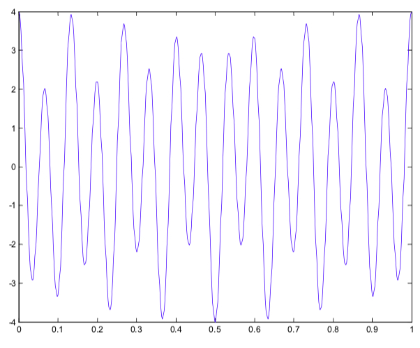
All waveforms, no matter what you scribble or observe in the universe, are actually just the sum of simple sinusoids of different frequencies.
Explanation by 李家同

一個訊號
f (t) = cos( (2 pi) * 7 * t) + 3 cos( (2 pi) * 15 * t)
 |  |
在左邊,我們可以看到兩個尖端 , 一個在頻率 f =7 的地 方 , 一個在頻率 f =15 的地方.
大概說起來 , 傅葉爾轉換的理論是說,任何一個訊號 , 都是一大堆cosine函 數的和。
The Fourier transform G(f) and the inverse Fourier transform g(t):

where:
- t stands for time
- f stands for frequency
- g denotes the signal in time domain
- G denotes the signal in frequency domain
Fourier Transforms are performed using complex numbers. The complex form of the equations makes things a lot simpler and more elegant.

Therefore, the exponential term in FT can also be written as:
Cos(2.pi.f.t) + j * Sin(2.pi.f.t)
Please take a closer look at equation of FT:
The signal g(t), is multiplied with an exponential term, at some certain frequency "f" , and then integrated over ALL TIMES !!!
- If the result of this integration (which is nothing but some sort of infinite summation) is a large value, then we say that: the signal x(t), has a dominant spectral component at frequency "f". This means that, a major portion of this signal is composed of frequency f.
- If the integration result is a small value, then this means that the signal does not have a major frequency component of f in it.
- If this integration result is zero, then the signal does not contain the frequency "f" at all.
This is why Fourier transform is not suitable if the signal has time varying frequency, i.e., the signal is non-stationary.
Consider that there are 2 signals with the same 5 frequency components of 5, 10, 20, and 50 Hz and the corresponding FT:
| 4 frequencies occur always occur |  |  |
| 4 frequencies occur at different time |  |  |
You can see how the below starts to look more like a square wave the more sin() terms, or frequencies, you add.

The point is that any signal can be decomposed into an equation with just sin() and cos() waves being added together, resulting in a frequency graph.
Once you do a Fourier Transform on a signal you can reduce noise, compress data, modulate, filter, encode and more.
Once the signal has been dealt with in the frequency domain, you can do the inverse Fourier Transform from the the signal's
frequency domain back to the time domain.
The Short Term Fourier Transform
In STFT, the signal is divided into small enough segments, where these segments (portions) of the signal can be assumed to be stationary. For this purpose, a window function "w" is chosen. The width of this window must be equal to the segment of the signal where its stationarity is valid.
Let's suppose that the width of the window is "T" s. At this time instant (t=0), the window function will overlap with the first T/2 seconds. The result of this transformation is the FT of the first T/2 seconds of the signal.
The problem with the STFT has something to do with the width of the window function that is used.
The problem here is that cutting the signal corresponds to a convolution between the signal and the cutting window.
Fourier Transforms (scipy.fftpack)
Multi-resolution Analysis and The Continuous Wavelet Transform
The multiresolution analysis (MRA), as implied by its name, analyzes the signal at different frequencies with different resolutions.
This approach makes sense especially when the signal at hand has high frequency components for short durations and low frequency components for long durations.
The continuous wavelet transform was developed as an alternative approach to the short time Fourier transform to overcome the resolution problem.
The wavelet analysis is done in a similar way to the STFT analysis, in the sense that the signal is multiplied with a function, similar to the window function in the STFT, and the transform is computed separately for different segments of the time-domain signal.
In wavelet analysis the use of a fully scalable modulated window solves the signal-cutting problem.
The window is shifted along the signal and for every position the spectrum is calculated. Then this process is repeated many times with a slightly shorter (or longer) window for every new cycle.
The continuous wavelet transform or CWT. More formally it is written as:( Reference: "A Really Friendly Guide to Wavelets" by c.valens@mindless.com )

We usually consider only positive scale factor s > 0. The wavelets are dilated when the scale s > 1 and are contracted when s < 1. It is important to note that in (1), (2) and (3) the wavelet basis functions are not specified. This is a difference between the wavelet transform and the Fourier transform, or other transforms. The theory of wavelet transforms deals with the general properties of the wavelets and wavelet transforms only.
The term wavelet means a small wave .
- The smallness refers to the condition that this (window) function is of finite length (compactly supported).
- The wave refers to the condition that this function is oscillatory.
The wavelets generated from the same mother wavelet have different scales s and locations τ, but all have the identical shape.
The base of the wavelet transform, the wavelets, satisfy an admissible condition so that the original signal can be reconstructed by the inverse wavelet transform.

The second basic property is related to the fact that the wavelet transform should be a local operator in both time and frequency domains. Hence, the regularity condition is usually imposed on the wavelets so that the wavelet transform decrease fast with decreases of the scale.
The Scale
The parameter scale in the wavelet analysis is similar to the scale used in maps. As in the case of maps,
- high scales correspond to a non-detailed global view (of the signal)
- low scales correspond to a detailed view
- low frequencies (high scales) correspond to a global information of a signal (that usually spans the entire signal)
- high frequencies (low scales) correspond to a detailed information of a hidden pattern in the signal (that usually lasts a relatively short time)

The above are dilated or contracted versions of the same cosine function. Larger scales correspond to dilated (or stretched out) signals and small scales correspond to contracted signals.
Computation of CWT
Let x(t) is the signal to be analyzed. The mother wavelet is chosen to serve as a prototype for all windows in the process. The Morlet wavelet and the Mexican hat function are two candidates
For convenience, the analysis will start from high frequencies and proceed towards low frequencies.
- The procedure will be started from scale s=1 and τ=0
- The wavelet is placed at the beginning of the signal at the point which corresponds to time=0.(τ=0)
- The wavelet function at scale s=1 is multiplied by the signal and then integrated over all times.
- The result of the integration is then multiplied by the constant number 1/sqrt(s).
- The final result is the value of the transformation, i.e., the value of the continuous wavelet transform at time zero and scale s=1.
- The wavelet at scale s=1 is then shifted towards the right by τ amount to the location t=τ. Then, the above procedure is used to get the transform value at t=τ , s=1 in the time- frequency plane.
- This procedure is repeated until the wavelet reaches the end of the signal.
- Then, s is increased by a small value and the above procedure is repeated for every value of s.
- When the process is completed for all desired values of s, the CWT of the signal has been calculated.
The figures below illustrate the entire process step by step. The signal (yellow) and the wavelet function (blue) are shown for four different values of τ, 2, 40, 90, and 140.

At every location, it is multiplied by the signal. Obviously, the product is nonzero only where the signal falls in the region of support of the wavelet, and it is zero elsewhere.
By shifting the wavelet in time, the signal is localized in time, and by changing the value of s, the signal is localized in scale (frequency).
If the signal has a spectral component that corresponds to the current value of s (which is 1 in this case), the product of the wavelet with the signal at the location where this spectral component exists gives a relatively large value. If the spectral component that corresponds to the current value of s is not present in the signal, the product value will be relatively small, or zero.
Note how the window width changes with increasing scale (decreasing frequency). As the window width increases, the transform starts picking up the lower frequency components.

As a result, for every scale and for every time (interval), one point of the time-scale plane is computed.
The computations at one scale construct the rows of the time-scale plane, and the computations at different scales construct the columns of the time-scale plane.
Consider the non-stationary signal composed of 4 frequency components at 30 Hz, 20 Hz, 10 Hz and 5 Hz.

Introduction to Wavelet
byFengxiang Qiao, Ph.D.
Texas Southern University
Overview
- Wavelet A small wave
- Wavelet Transforms
- frequency and duration
- Allow signals to be stored more efficiently than by Fourier transform
- Be able to better approximate real-world signals
- Well-suited for approximating data with sharp discontinuities
- “The Forest & the Trees”
- Notice gross features with a large "window“
- Notice small features with a small "window”
- Convert a signal into a series of wavelets Provide a way for analyzing waveforms, bounded in both
Historical Development
Time vs Frequency Domain Analysis Fourier Analysis
MATHEMATICAL TRANSFORMATION
- Why To obtain a further information from the signal that is not readily available in the raw signal.
- Raw Signal Normally the time-domain signal
- Processed Signal A signal that has been "transformed" by any of the available mathematical transformations
- Fourier Transformation The most popular transformation
TIME-DOMAIN SIGNAL
- The Independent Variable is Time
- The Dependent Variable is the Amplitude
- Most of the Information is Hidden in the Frequency Content
FREQUENCY TRANSFORMS
- Why Frequency Information is Needed Be able to see any information that is not obvious in time-domain
- Types of Frequency Transformation Fourier Transform, Hilbert Transform, Short-time Fourier Transform, Wigner Distributions, the Radon Transform, the Wavelet Transform ...
FREQUENCY ANALYSIS
- Frequency Spectrum
- Be basically the frequency components (spectral components) of that signal
- Show what frequencies exists in the signal
- Fourier Transform (FT)
- One way to find the frequency content
- Tells how much of each frequency exists in a signal
STATIONARITY OF SIGNAL
- Stationary Signal
- Signals with frequency content unchanged in time
- All frequency components exist at all times
- Non-stationary Signal
- Frequency changes in time
- One example: the “Chirp Signal”
- FT Only Gives what Frequency Components Exist in the Signal
- The Time and Frequency Information can not be Seen at the Same Time
- Time-frequency Representation of the Signal is Needed


SFORT TIME FOURIER TRANSFORM (STFT)
- To analyze only a small section of the signal at a time -- a technique called Windowing the Signal.
- The Segment of Signal is Assumed Stationary
- A 3D transform

DRAWBACKS OF STFT
- Unchanged Window
- Dilemma of Resolution
- Narrow window: poor frequency resolution
- Wide window: poor time resolution
- Heisenberg Uncertainty Principle In Physics the principle goes along the lines of: you can know where a particle is or how fast it is going, but not both. The graph below is a representation of the uncertainty principle. The position of the ball is on the x-axis and the sped of the ball is on the y-axis. The red dot shows the actual speed and position on the graph:
 Each box has the same area. For instance the blue box is tall and thin. The fact that it is thin around the position of the ball indicates that this measurement is pretty certain of the position. However to keep the box the same area, it has to stretch out along the y-axis, indicating that it is unsure of the value for the speed. This amount of uncertainty is also called resolution of the measurement. The time-frequency has this minimum amount of uncertainty too:
  You can know the moment in time you want to find the frequency for (like the blue box), but because there is a minimum uncertainty, the box of has to stretch out across frequency, meaning that you are unsure of the frequency at that moment in time.
 The below picture shows the time signal of sin(x**2) and the right picture is what a ‘Windowed Fourier Transform’ thinks the frequency is over time. You can see by the thick dark shaded line that it is uncertain what the frequency is at any moment in time, even though the original signal does have an exact frequency at each moment.

With the above, we can understand how the Fourier Transform has a lack of resolution between the frequency and time domain.
Fourier vs Wavelet Transforms
Wavelets are useful because they are limited in time and frequency.

When a signal is deconstructed into wavelets rather than sin() and cos(), it is called a Wavelet Transform. The graph that can be analyzed after the transform is in the wavelet domain, rather than the frequency domain.
How do wavelets handle low and high frequencies? This is handled by something called the scale of the wavelet.

MULTIRESOLUTION ANALYSIS (MRA)
Wavelet Transform
- An alternative approach to the short time Fourier transform to overcome the resolution problem
- Similar to STFT: signal is multiplied with a function
Multiresolution Analysis
- Analyze the signal at different frequencies with different resolutions
- Good time resolution and poor frequency resolution at high frequencies
- Good frequency resolution and poor time resolution at low frequencies
- More suitable for short duration of higher frequency; and longer duration of lower frequency components
ADVANTAGES OF WT OVER STFT
- Width of the Window is Changed as the Transform is Computed for Every Spectral Components
- Altered Resolutions are Placed
Wavelet Analysis
PRINCIPLES OF WAELET TRANSFORM
- Split Up the Signal into a Bunch of Signals
- Representing the Same Signal, but all Corresponding to Different Frequency Bands
- Only Providing What Frequency Bands Exists at What Time Intervals
DEFINITION OF CONTINUOUS WAVELET TRANSFORM

SCALE
- S>1: dilate the signal
- S<1: compress the signal
- Low Frequency -> High Scale -> Non- detailed Global View of Signal -> Span Entire Signal
- High Frequency -> Low Scale -> Detailed View Last in Short Time
- Only Limited Interval of Scales is Necessary
COMPUTATION OF CWT
- Step 1: The wavelet is placed at the beginning of the signal, and set s=1 (the most compressed wavelet);
- Step 2: The wavelet function at scale “1” is multiplied by the signal, and integrated over all times; then multiplied by1 s ;
- Step 3: Shift the wavelet to t= τ , and get the transform value at t= τ and s=1;
- Step 4: Repeat the procedure until the wavelet reaches the end of the signal;
- Step 5: Scale s is increased by a sufficiently small value, the above procedure is repeated for all s;
- Step 6: Each computation for a given s fills the single row of the time-scale plane;
- Step 7: CWT is obtained if all s are calculated.
Time–frequency analysis
Time–frequency analysis studies a two-dimensional signal – a function whose domain is the two-dimensional real plane, obtained from the signal via a time–frequency transform.
The mathematical motivation for this study is that functions and their transform representation are often tightly connected, and they can be understood better by studying them jointly, as a two-dimensional object, rather than separately.
RESOLUTION OF TIME and FREQUENCY
Tools and Software
Typical Applications
Summary
References
An Introduction to Wavelets
by Amara GrapsIEEE Computational Science and Engineering, Summer 1995, vol. 2, num. 2, published by the IEEE Computer Society
2. HISTORICAL PERSPECTIVE
2.1. PRE-1930

3. FOURIER ANALYSIS
A Fourier series is a way to decompose any periodic function or periodic signal into the sum of a (possibly infinite) set of simple oscillating functions, namely sines and cosines (or, equivalently, complex exponentials).
Fourier analysis is the study to represent functions by sums of simpler trigonometric functions.
In the sciences and engineering, the process of decomposing a function into oscillatory components is often called Fourier analysis, while the operation of rebuilding the function from these pieces is known as Fourier synthesis.
3.1. FOURIER TRANSFORMS
The Fourier transform (FT) decomposes a function of time (a signal) into the frequencies that make it up.
The Fourier transform is called the frequency domain representation of the original signal.

The transform works by first translating a function in the time domain into a function in the frequency domain. The signal can then be analyzed for its frequency content because the Fourier coefficients of the transformed function represent the contribution of each sine and cosine function at each frequency.
3.2. DISCRETE FOURIER TRANSFORMS
The discrete Fourier transform (DFT) estimates the Fourier transform of a function from a finite number of its sampled points.

3.3. WINDOWED FOURIER TRANSFORMS
If f(t) is a non-periodic signal, it cannot be represented by sum of sine and cosine functions.
The windowed Fourier transform (WFT) chop the signal into sections and each section is analyzed for its frequency content separately.
This windowing is accomplished via a weight function that places less emphasis near the interval’s endpoints than in the middle. The effect of the window is to localize the signal in time.
A wide window gives better frequency resolution but poor time resolution. A narrower window gives good time resolution but poor frequency resolution.
This is one of the reasons for the creation of the wavelet transform and multi-resolution analysis, which can give good time resolution for high-frequency events and good frequency resolution for low-frequency events, the combination best suited for many real signals.
Let's look at the following example.
Using the following sample signal x(t) that is composed of a set of four sinusoidal waveforms joined together in sequence. Each waveform is only composed of one of four frequencies :10, 25, 50, 100 Hz.

Then it is sampled at 400 Hz. ( > 2*fmax(100)).
A spectrogram is a visual representation of the spectrum of frequencies of signals as they vary with time.
The following spectrograms were produced for 4 time window size in Short-time Fourier transform:
- 25 ms
- 125 ms
- 375 ms
- 1000 ms


At the other end of the scale, the 1000 ms window allows the frequencies to be precisely seen but the time between frequency changes is blurred.
3.4. FAST FOURIER TRANSFORMS
Big O notation is used to describe the asymptotic behavior of functions.
For ex., the time (or the number of steps) it takes to complete a problem of size n is given by
T(n)=4*n*n -2n + 2
T(n) = O(n*n).
4. WAVELET TRANSFORMS VERSUS FOURIER TRANSFORMS
6. WAVELET ANALYSIS
6.1. THE DISCRETE WAVELET TRANSFORM
An orthogonal wavelet basis is defined as:

The variables s and l are integers that scale and dilate the mother function Φ to generate wavelets.
Notice that the mother functions are rescaled, or “dilated” by powers of two, and translated by integers.
Once we know about the mother functions, we know everything about the basis.
Wavelets with applications in signal and image processing
by Adhemar Bultheel and Daan HuybrechsOctober 2011
Chapter 1 Introduction
1.1 The first example
Consider a signal consisting of 8 samples (top left):
x = (x1,x2,...,x8) = (1,3,5,7,2,−1,−3,−2)
The space V0 of all such signals is in fact the space R8, namely the space of all 8-tuples.
Next we replace every 2 samples by their average, we also have to store the error, i.e., the difference between the original signal and the averaged signal.
The averaged signal is denoted x(−1) and the difference signal is denoted y(−1). Thus,
x = x(−1) + y(−1).

Learning to swim in a sea of wavelets
by Adhemar Bultheel1 History
2 Motivation
Introduction to Data Compression
by Khalid SayoodChapter 15 Wavelets
15.2 Introduction
Wavelets are being used in a number of different applications. Depending on the application, different aspects of wavelets can be emphasized.
The practical implementation of wavelet compression schemes is very similar to that of subband coding schemes.
As in the case of subband coding, we decompose the signal using analysis filter banks. The outputs of the filter banks are downsampled, quantized, and encoded. The decoder decodes the coded representations, upsamples, and recomposes the signal using a synthesis filter bank.
Given a function f(t), we can find its Fourier transform F(ω) by integration.

Integration is an averaging operation; therefore, the analysis we obtain, using the Fourier transform, is in some sense an “average” analysis, where the averaging interval is all of time.
Thus, by looking at a particular Fourier transform, we can say, for example, that there is a large component of frequency 10 kHz in a signal, but we cannot tell when in time this component occurred. In other words, Fourier analysis provides excellent localization in frequency and none in time.
It should be noted that both f (t) and F(ω) represent the same function, and all the information is present in each representation. However, each representation makes different kinds of information easily accessible.
If we want to know when in time the particular frequency components occurred. One way to obtain this information is via the short-term Fourier transform (STFT).

With the STFT, we break the time signal f(t) into pieces of length T and apply Fourier analysis to each piece.
If we simply chopped the function into pieces, we could get distortion in the form of boundary effects. In order to reduce the boundary effects, we window each piece before we take the Fourier transform.
If the window function g(t) is a Gaussian, the STFT is called the Gabor transform.
The problem with the STFT is the fixed window size.
In order to obtain the low-pass component at the beginning of the function, the window size should be at least t0 so that the window will contain at least one cycle of the low-frequency component. However, a window size of t0 or greater means that we will not be able to accurately localize the high-frequency spurt.
Therefore, a large window in the time domain corresponds to a narrow filter in the frequency domain, a narrow time window is for high frequency filtering.
A sinusoidal wave has a perfectly clearly determined frequency, but it is spread over the infinitely long time axis. At the other extreme is a delta function, which is nicely compressed to a point on the time axis but contains a mixture of all frequencies.
Time-bandwidth product is the product of the duration of a signal and its spectral width.
Generally, signals of short duration have wide spectral width and vice versa. The time-bandwidth product for actual signals will vary but there will always be a minimum time-bandwidth product for a certain desired effect. In communications over a channel, transmitting a certain amount of data over a given bandwidth requires a certain time. The time-bandwidth product measures how well we use the available bandwidth for a given channel. This dilemma is formalized in the uncertainty principle.

The resolution of time and frequency for a signal is on the opposite.
The basic idea behind wavelets is that the lower frequency functions cover a longer time interval, while the higher frequency functions cover a shorter time interval.
15.3 Wavelets
Mathematically, we can scale a function f (t) by replacing t with t/a, where the parameter a governs the amount of scaling.


If we define the norm of a function f(t):

scaling obviously changes the norm of the function:

This is because the time scaling changes the occurrence of the signal.
If we want the scaled function to have the same norm as the original function, we need to multiply it by 1/√a. Transformations that change the size of an object but not its shape are often referred to as dilation, which is a term we will use interchangeably with scaling in our discussion.
We can use the translation and scaling operations to generate a family of functions from a single function. Thus, given a mother function ψ(t), we can generate a whole family of

If this family of functions satisfies certain properties we can use them to represent signals of interest in a manner similar to the Fourier basis functions. Unlike the Fourier basis functions, because these functions are localized in time and frequency we can use them without giving up all the temporal information contained in the original function.
Coefficients with respect to these functions is obtained from the inner product of f(t) with the wavelet functions:

If a and b are continuous, then this is called the continuous wavelet transform (CWT).
We can recover the function f(t) by the wavelets and its CWT:

For Cψ to be finite, we need

This means that the mother wavelet must have zero mean.
We would also like the wavelets to have finite energy

These requirements mean that the energy is concentrated in a narrow frequency band
The discrete versions of the scaling and translating parameters (a, b) have to be related to each other, because if the scale is such that the basis functions are narrow, the translation step should be correspondingly small and vice versa. There are a number of ways we can choose these parameters. The most popular approach is to select a and b according to
We first obtain a series representation where the basis functions are continuous functions of time with discrete scaling and translating parameters a and b. The discrete versions of the scaling and translating parameters have to be related to each other, because if the scale is such that the basis functions are narrow, the translation step should be correspondingly small and vice versa. The most popular approach is to select a and b according to

where m and n are integers and a0 and b0 are constants.
For a0=2 and b0 =1, we have

The wavelet coefficients are given by

The function f(t) can be reconstructed from the wavelet coefficients by

Wavelets come in many shapes. One of the simplest wavelets is the Haar wavelet.


15.4 Multiresolution Analysis and the Scaling Function
Consider the Haar scaling function:

and let's define

If f(t) is any piecewise continuous function that is constant in the interval [k, k + 1) for all k,
then f(t) can be represented by a linear combination of the set {φk(t)}

This is called the span of the set { φk(t)}, or Span{ φk(t)}.
If we want to represent functions at a higher resolution, say functions that are required to be constant over only half a unit interval, we can use a dilated version of the φk(t) function.

For the Haar example,

We can use this to represent all functions that are constant over intervals [k/2, (k + 1)/2) for all k.

Consider the following function:

This function can be approximated by different scaled Harr function:


We can obtain a more refined approximation, or an approximation at a higher resolution,

Notice that we need twice as many coefficients at this resolution compared to the previous resolution. ( The frequency doubled as time spacing decreased )
Continuing in this manner, we can get higher and higher resolution approximations of f(t) with

If the highest frequency component of a signal is at f0 Hz, we need 2 f0 samples per second to accurately represent it.
15.5 Implementation Using Filters
15.5.2 Families of Wavelets
There is an infinite number of possible wavelets.
Which one is best depends on the application.
15.6 Biorthogonal Wavelets
In this section, we will describe what biorthogonal wavelets are and why we would want to use them rather than orthogonal wavelets in image compression applications.

留言