Deep Learning From the Scratch
ゼロから作るDeep Learning
Code accompanying the book
――Pythonで学ぶディープラーニングの理論と実装
- 斎藤 康毅 著
- 2016年09月 発行
1 Python入門
1.2.3 Anaconda套裝版本管理
ANACONDA CHEAT SHEET:
- Why do I need Anaconda? Installing Python from scratch is no joy. Many scientific packages require a specific version of Python or R computer language along with many dependencies. It's hard to keep packages from interacting with each other, and harder to keep them all updated. Anaconda makes getting and maintaining all these packages quick and easy. The open source version of Anaconda is an easy-to-install high performance Python and R distribution with a package manager, environment manager and collection of 720+ open source packages with free community support.
- Then what is Miniconda? It's Anaconda without the collection of 720 open source packages. With Miniconda you download only the packages you want with the conda command, "conda install PACKAGENAME"
- Will it work on my machine? Yes, Anaconda is available for Windows, OS X or Linux, 32- or 64-bit, 400 MB HD available. Miniconda same but needs only 3 MB HD.
- Quick Install It docs.continuum.io/anaconda/install Go to the installed folder (\ProgramData\Anaconda3):
- python
- Scripts/conda
- Packaged included in Anaconda 4+, or get with "conda install PACKAGENAME"
- NumPy | numpy.org N-dimensional array for numerical computation
- SciPy | scipy.org Collection of numerical algorithms and toolboxes, including signal processing and optimization
- MatPlotLib | matplotlib.org Plotting library for Python
- Pandas | pandas.pydata.org Powerful Python data analysis toolkit
- Seaborn | stanford.edu/~mwaskom/software/seaborn/ Statistical data visualization
- Bokeh | bokeh.pydata.org Interactive web visualization library
Start jupyter notebook on Ubuntu:
  cd ~/anaconda3
  jupyter notebook
1.3.2 Data Type
type()1.3.4 List
# a = [1, 2, 3, 4 ]
#len(a)
4
# a[0:2] = a[0], a[1]
[1, 2]
a[:3] = a[0], a[1], a[2]
a[1:] = a[1], a[2], a[3], a[4]
a[-1] = a[3]
a[-2] = a[2]
1.3.5 Dictionary
man={'age': 49}
man['age'] # 49
1.3.6 Boolean
True
False
Operations: and, or, nor
1.4.2 Class
class 類別名稱:
    def __init__(self, 參數, ...): # constructor
        ...
    def 方法1(self, 參數, ...): # method
        ...
1.5 NumPy
NumPy的類別numpy.array提供許多計算陣列或矩陣的方法.
1.5.1 import numpy as np
1.5.2 Create NumPy Array( numpy.ndarray )
np.array()接受list為參數以產生NumPy的陣列
1.5.3 NumPy對陣列的算術運算
算術運算是針對陣列的元素
兩陣列做運算時, 陣列中元素的數目必須相同, 運算是在相對應位置的元素間執行.(不是linear algebra的inner produce)
1.5.4 NumPy的多維陣列
A=np.array( [[1,2],[3,4]])
矩陣的維度可用方法shape()得知, 元素的資造型別可用方法dtype()得知.
Broadcast
When operating on two arrays, NumPy compares their shapes element-wise. It starts with the trailing dimensions, and works its way forward. Two dimensions are compatible when
- they are equal, or
- one of them is 1
Arrays do not need to have the same number of dimensions. For example, if you have a 256x256x3 array of RGB values, and you want to scale each color in the image by a different value, you can multiply the image by a one-dimensional array with 3 values.
Lining up the sizes of the trailing axes of these arrays according to the broadcast rules, shows that they are compatible:
Image  (3d array): 256 x 256 x 3
Scale  (1d array):             3
Result (3d array): 256 x 256 x 3
When either of the dimensions compared is one, the other is used. In other words, dimensions with size 1 are stretched or “copied” to match the other.
A      (4d array):  8 x 1 x 6 x 1
B      (3d array):      7 x 1 x 5
Result (4d array):  8 x 7 x 6 x 5
1.5.6 存取元素
flatten()可以把矩陣轉成一維陣列
A=A.flatten()
1.6 Matplotlib
1.6.1 繪圖表
matplotlib.pyplot provides a MATLAB-like plotting framework.
import numpy as np
import matplotlib.pyplot as plt

x = np.arange(0, 5, 0.1);
y = np.sin(x)
plt.plot(x, y)
numpy.arange([start, ]stop, [step, ]dtype=None)
numpy.sin(x, /, out=None, *, where=True, casting='same_kind', order='K', dtype=None, subok=True[, signature, extobj]) =
x : array_like. Angle, in radians (2 \pi rad equals 360 degrees).
1.6.2 more on pyplot
1.6.3 Show Image
pyplot提供顯示影像的方法imshow().
matplotlib.pyplot.imshow(X, cmap=None, norm=None, aspect=None, interpolation=None, alpha=None, vmin=None, vmax=None, origin=None, extent=None, shape=None, filternorm=1, filterrad=4.0, imlim=None, resample=None, url=None, hold=None, data=None, **kwargs)
X : array_like, shape (n, m) or (n, m, 3) or (n, m, 4)
Display the image in X to current axes. X may be an array or a PIL image. If X is an array, it can have the following shapes and types:
MxN – values to be mapped (float or int)
MxNx3 – RGB (float or uint8)
MxNx4 – RGBA (float or uint8)
The value for each component of MxNx3 and MxNx4 float arrays should be in the range 0.0 to 1.0. MxN arrays are mapped to colors based on the norm (mapping scalar to scalar) and the cmap (mapping the normed scalar to a color).
要載入影像, 可以透過matplotlib.image的imread(), matplotlib only supports PNG images.
2 感知器(Perception)
Deep learning is a subfield of Machine Learning, and Machine Learning is a subfield of Artificial Intelligence.
2.1 何謂感知器
“a machine which senses, recognizes, remembers, and responds like the human mind” is called the a Perceptron.
The perceptron is an algorithm for learning a binary classifier f(x): a function that maps its input x to an output binary value

where w is a vector of real-valued weights, w x is the dot product
The value of f(x) (0 or 1) is used to classify x as either a positive or a negative instance, in the case of a binary classification problem.
b is the bias. The bias shifts the decision boundary away from the origin and does not depend on any input value.

In the context of neural networks, a perceptron is an artificial neuron using the Heaviside step function as the activation function. The perceptron algorithm is also termed the single-layer perceptron.
Perceptron is used in supervised learning. It helps to classify the given input data.
我們思考感知器的模型(parameters), 收集可學習的資料, 再用人工方式決定weight.
In machine learning, computer decides the weight.
2.2 logic感知器
同樣的感知器架構, 不同的參數會決定感知器的行為(輸出)
AND gate
| x1 | x2 | f(x) |
|---|---|---|
| 0 | 0 | 0 |
| 1 | 0 | 0 |
| 0 | 1 | 0 |
| 1 | 1 | 1 |
NAND gate, OR gate
| x1 | x2 | f(x) |
|---|---|---|
| 0 | 0 | 1 |
| 1 | 0 | 1 |
| 0 | 1 | 1 |
| 1 | 1 | 0 |
| x1 | x2 | f(x) |
|---|---|---|
| 0 | 0 | 0 |
| 1 | 0 | 1 |
| 0 | 1 | 1 |
| 1 | 1 | 1 |
2.3 實作感測器
2.3.1 簡單實作
def AND(x1, x2):
    w1, w2, theta = 0.5, 0.5, 0.7
    tmp = x1*w1 + x2*w2
    if ( tmp <= theta ):
        return 0
    elif tmp > theta:
        return 1
2.3.2 使用NumPy並導入offset
import numpy as np

x = np.array([0, 1])
w = np.array([0.5, 0.5])
b = -0.7
tmp = np.sum(w * x) + b
2.3.3 重新實作logic gate
def AND(x1, x2):
    x = np.array([x1, x2])
    w = np.array([0.5, 0.5])
    b = -0.7
    tmp = np.sum(w *x) + b
    if (tmp <= 0):
        return 0
    else:
        return 1

def NAND(x1, x2):
    x = np.array([x1, x2])
    w = np.array([-0.5, -0.5])
    b = 0.7
    tmp = np.sum(w *x) + b
    if (tmp <= 0):
        return 0
    else:
        return 1

def OR(x1, x2):
    x = np.array([x1, x2])
    w = np.array([0.5, 0.5])
    b = -0.2
    tmp = np.sum(w *x) + b
    if (tmp <= 0):
        return 0
    else:
        return 1
所以,AND, OR和NAND gate是結構相同的感知器, 只有weight和offset不同.
2.4 感知器的極限
單一感知器的輸出無法以線性方程式分隔輸入來判定結果.
2.4.1 XOR Gate
XOR無法以線性方程式由輸入來判定結果
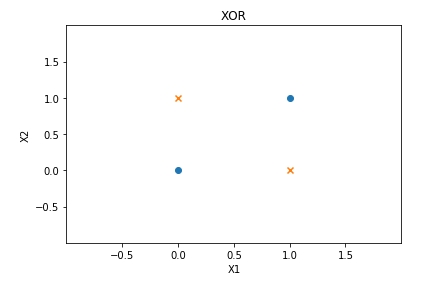
2.4.2 線性與非線性

2.5 多層感知器
2.5.1 以現有的gate組合

2.5.2 以多層實作XOR gate
def XOR(x1, x2):
    s1 = NAND(x1, x2)
    s2 = OR(x1, x2)
    y = AND( s1, s2)
    return y
此為雙層感知器.
2.6 由NAND gate可製作computer
理論上, 藉由雙層感知器的組合就可以做成computer
3 神經網路

previous Neuron               current Neuron
-------------------------    -----------------------------------------
axon   dendrite  synapse                cell                output axon
軸突    樹突       突觸
====   ========  ========    ============================  =============
          Xi      Wij         sum( Xi * Wij + Bij ) + act
神經網路是為了要能自動地學習以找出最佳的weight及offset.
3.1 Multi-Layer Neural Networks

Ronald Williams published a paper “Learning representations by back-propagating errors”, which introduced:
- Backpropagation A procedure to repeatedly adjust the weights so as to minimize the difference between actual output and desired output
- Hidden Layers Neuron nodes stacked in between inputs and outputs, allowing neural networks to learn more complicated features (such as XOR logic)
3.2 Activation Function


- Inputs are fed into the perceptron
- Weights are multiplied to each input
- Summation and then add bias
- Activation function is applied. Note that here we use a step function, but there are other more sophisticated activation functions like :
- sigmoid
- hyperbolic tangent (tanh)
- rectifier (relu)
- ...
- Output is either triggered as 1, or not, as 0. Note we use y hat to label output produced by our perceptron model
Why does deep learning/architectures only use the non-linear activation function in the hidden layers?
Without a nonlinear activation function, the neural network is calculating linear combinations of values.
3.2.1 sigmoid

3.2.2 實作step function
def step_function(x):
    if (x >0):
        return 1
    else:
        return 0
To process the input array,
import numpy as np

def step_function(x):
    y = x > 0                     # NumPy array 執行不等運算是針對陣列中所有的元素執行不等運算
    return y.astype(np.int)       # astype() copy of the array, cast to a specified type. Convert the Boolean array to the integer array.


x = np.array([-1.0, 1.0, 2.0])
y = step_function(x)
3.2.3 The plot of the step function
import numpy as np
import matplotlib.pylab as plt

def step_function(x):
    return np.array( x>0, dtype=np.int)

x = np.arange(-5.0, 5.0, 0.1)
y = step_function(x)
plt.plot(x, y)
plt.ylim(-0.1, 1.1)
plt.show()
3.2.4 實作sigmoid function
import numpy as np
import matplotlib.pylab as plt

def sigmoid(x):
    return 1 / (1 + np.exp(-x) )

x = np.arange( -5.0, 5.0, 0.1)
y = sigmoid(x)
plt.plot(x, y)
plt.ylim(-0.1, 1.1)
plt.show()
3.2.5 step 和 sigmoid 函數的比較
step函數沒有可用的微分(0 或不可微分), 無法做back propagation.
With the step function, a small change in any weight in the input layer of our perceptron network could possibly lead to one neuron to suddenly flip from 0 to 1, which could again affect the hidden layer’s behavior, and then affect the final outcome.

We want a learning algorithm that could improve our neural network by gradually changing the weights, not by flat-no-response or sudden jumps.
sigmoid函數特性:
- Sigmoid function 產生的結果是平滑的.
- Sigmoid function 產生的結果可以是實數
3.2.6 非線性函數
線性函數的組合,其輸出仍然是和輸入呈現性相關的, 因此增加網路的層數是沒有意義的.
3.2.7 ReLU (Rectified Linear Unit)函數
輸入超過0, 輸出結果就是輸入; 輸入小於0就輸出0
def relu(x):
    return np.maximum(0, x)    # Compare two arrays and returns a new array containing the element-wise maxima.
3.3 多微陣列的運算
了解NumPy對於多維陣列的運算
3.3.1 多維的陣列
NumPy’s main object is the homogeneous multidimensional array.
It is a table of elements (usually numbers), all of the same type, indexed by a tuple of positive integers. In NumPy dimensions are called axes.
The number of axes is rank.
For example, the coordinates of a point in 3D space [1, 2, 1] is an array of rank 1, because it has one axis. That axis has a length of 3.
In the example pictured below,
[[ 1., 0., 0.],
 [ 0., 1., 2.]]
the array has rank 2 (it is 2-dimensional). The first dimension (axis) has a length of 2, the second dimension has a length of 3.
二維陣列被稱為矩陣.
NumPy’s array class is called ndarray. It is also known by the alias array.
Note that numpy.array is not the same as the Standard Python Library class array.array, which only handles one-dimensional arrays and offers less functionality.
The more important attributes of an ndarray object are:
- ndarray.ndim the number of axes (dimensions) of the array. In the Python world, the number of dimensions is referred to as rank.
- ndarray.shape the dimensions of the array. This is a tuple of integers indicating the size of the array in each dimension. For a matrix with n rows and m columns, shape will be (n,m). The length of the shape tuple is therefore the rank, or number of dimensions, ndim.
- ndarray.size the total number of elements of the array. This is equal to the product of the elements of shape.
- ndarray.dtype an object describing the type of the elements in the array. One can create or specify dtype’s using standard Python types. Additionally NumPy provides types of its own. numpy.int32, numpy.int16, and numpy.float64 are some examples.
- ndarray.itemsize the size in bytes of each element of the array. For example, an array of elements of type float64 has itemsize 8 (=64/8), while one of type complex32 has itemsize 4 (=32/8). It is equivalent to ndarray.dtype.itemsize.
- ndarray.data the buffer containing the actual elements of the array. Normally, we won’t need to use this attribute because we will access the elements in an array using indexing facilities.
import numpy as np

A = np.array([1,2,3,4]) # 建立一維陣列

print(A)
[1 2 3 4]

np.ndim(A)   # 取得陣列的維度
Out[4]: 1

A.shape      # 取得陣列的形狀
Out[5]: (4,)

A.shape[0]
Out[6]: 4

B = np.array([[1,2],[3,4],[5,6]])  # 建立二維陣列

print(B)
[[1 2]
 [3 4]
 [5 6]]

np.ndim(B)   # 取得陣列的維度
Out[10]: 2

B.shape      # 取得陣列的形狀
Out[11]: (3, 2)
3.3.2 矩陣的乘積
指的是內積(dot product, inner product).
兩個2維矩陣要相乘,第一個矩陣的第1維度的元素數目要和第二個矩陣的第0維度的元素數目相同, 才能計算.


要顯示一個矩陣有多少個row及column, 是以rows × columns表示
當我們做矩陣乘法時:
- 第一個矩陣的columns必須等於第二個矩陣的rows
- 結果的rows和第一個矩陣的rows一樣, 而且columns和第二個矩陣一樣.

3.3.3 執行神經網路的乘積
要考慮到輸入(X), 權值(W) 及輸出矩陣(Y)的形狀.
特別是X和W對應的維度元素數量要相同.

The best way to think about NumPy arrays is that they consist of two parts,
- a data buffer which is just a block of raw elements
- a view which describes how to interpret the data buffer.
For example, if we create an array of 12 integers:
 a = np.arange(12)
 a
array([ 0,  1,  2,  3,  4,  5,  6,  7,  8,  9, 10, 11])
 a.shape
(12,)
If we reshape an array, this doesn't change the data buffer. Instead, it creates a new view that describes a different way to interpret the data. So after:
b = a.reshape((3, 4))
array([[ 0,  1,  2,  3],
       [ 4,  5,  6,  7],
       [ 8,  9, 10, 11]])
使用np.dot()可以計算多維陣列的內積:
import numpy as np

X = np.array([1,2])
X.shape
Out[5]: (2,)
W = np.array([[1,3,5],[2,4,6]])

print(W)
[[1 3 5]
 [2 4 6]]

W.shape
Out[9]: (2, 3)

Y = np.dot(X,W)

print(Y)
[ 5 11 17]
3.4 實作3層神經網路
3.4.1 確認符號
權重的表示法:
    (1)
  W
   1 2
- 右上方的數字 表示某個層的權重. 1代表第一層.
- 右下方的兩個數字 第1個數字表示前一層的第幾個神經元, 第2個數字表示下一層的第幾個神經元.

3.4.2 實作各層的訊號傳遞
輸入層到第一層:
 (1)       (1)    (1)
A    =  X W    + B
import numpy as np

X = np.array([1.0, 0.5])
W1 = np.array([[2.1, 0.3, 0.5], [0.2, 0.4, 0.6]])
B1 = np.array([0.1, 0.2, 0.3])


print(X.shape)
(2,)
print(W1.shape)
(2, 3)
print(B1.shape)
(3,)

A1 = np.dot(X,W1) + B1

print(A1)
[ 2.3  0.7  1.1]
在第一層神經元,他的輸出經由活化函數產生
Z1 = sigmoid(A1)
import matplotlib.pylab as plt

def sigmoid(x):
    return 1 / (1 + np.exp(-x) )


Z1 = sigmoid(A1)

print(Z1)
[ 0.90887704  0.66818777  0.75026011]
W2 = np.array([[0.1, 0.4], [0.2, 0.5], [0.3, 0.6]])
B2 = np.array([0.1, 0.2])

print(Z1.shape)
(3,)
print(W2.shape)
(3, 2)
print(B2.shape)
(2,)

A2 = np.dot(Z1, W2) + B2
Z2 = sigmoid(A2)
處理第2層的輸出到第3層的輸出, 最後一層的活化函數通常會和前面隱藏層的不同
此處設為恆等函數(為了讓執行過程跟前面兩層一樣)是不會改變任何值
最後的輸出結果def identify_function(x): return x
W3 = np.array([[0.1, 0.3], [0.2, 0.4]])
B3 = np.array([0.1, 0.2])
A3 = np.dot(Z2, W3) + B3

Y = identify_function(A3)

print(Y)
[ 0.32215832  0.707721  ]
3.4.3 實作整個過程
 import numpy as np

def init_network():
    network = {}
    network['W1'] = np.array([[0.1, 0.3, 0.5], [0.2, 0.4, 0.6]])
    network['b1'] = np.array([0.1, 0.2, 0.3])
    network['W2']= np.array([[0.1, 0.4], [0.2, 0.5], [0.3, 0.6]])
    network['b2'] = np.array([0.1, 0.2])
    network['W3']=np.array([[0.1,0.3], [0.2,0.4]])
    network['b3']=np.array([0.1, 0.2])
    return network

 def forward(network, x):
    W1, W2, W3 = network['W1'], network['W2'], network['W3']
    b1, b2, b3 = network['b1'], network['b2'], network['b3']
    a1 = np.dot(x, W1) + b1
    z1 = sigmoid(a1)
    a2 = np.dot(z1, W2) + b2
    z2 = sigmoid(a2)
    a3 = np.dot(z2,W3) + b3
    y = identify_function(a3)
    return y


network=init_network()
x=np.array([1.0,0.5])
y=forward(network, x)

print(y)
[ 0.31682708  0.69627909]
3.5 輸出層的設計:
Fundamentally, classification is about predicting a label and regression is about predicting a quantity.
- Classification predictive modeling is the task of approximating a mapping function (f) from input variables (X) to discrete output variables (y).
The output variables are often called labels or categories. - Regression predictive modeling is the task of approximating a mapping function (f) from input variables (X) to a continuous output variable (y).
A continuous output variable is a real-value, such as an integer or floating point value. These are often quantities, such as amounts and sizes.
3.5.1 softmax函數
Softmax is preferred in the output layer of deep learning models, especially when it is necessary to classify more than two(Sigmoid is used for binary classification). It allows determining the probability that the input belongs to a particular class by producing values in the range 0-1. So it performs a probabilistic interpretation.
若一個z向量有K個元素, 經過softmax的輸出後,第j個元素為 :


直接說明,softmax就是將原來輸入是3,1,-3通過softmax函數一作用,就映射成為(0,1)的值,而這些值的累和為1(滿足機率的性質),那麼我們就可以將它理解成機率,在最後選取輸出節點的時候,我們就可以選取機率最大(也就是值對應最大的)節點,作為我們的預測目標!
def softmax(a):
    exp_a = np.exp(a)
    sum = np.sum(exp_a)
    y = exp_a / sum
    return y
3.5.2 實作Softmax函數時的注意事項
The only accident that might happen is over/underflow in the exponentials.Overflow of a single or underflow of all elements of x will render the output more or less useless.
But it is easy to guard against that by using the identity:
softmax(x) = softmax(x + c)
Subtracting max(x) from x leaves a vector that has only non-positive entries, ruling out overflow and at least one element that is zero ruling out a vanishing denominator (underflow in some but not all entries is harmless).
def softmax(a):
    c = np.max(a)
    exp_a = np.exp(a-c)
    sum = np.sum(exp_a)
    y = exp_a / sum
    return y
3.6 辨識手寫的數字
3.6.1 MNIST資料集
The MNIST database (Modified National Institute of Standards and Technology database) has a training set of 60,000 examples(from approximately 250 writers), and a test set of 10,000 examples. The training set is used to teach the algorithm to predict the correct label, the integer, while the test set is used to check how accurately the trained network can make guesses.
In the machine learning world, this is called supervised learning, because we have the correct answers for the images we’re making guesses about. The training set can therefore act as a supervisor, or teacher, correcting the neural network when it guesses wrong.
It is a subset of a larger set available from NIST. The digits have been size-normalized and centered in a fixed-size image.
- Download the source
- Decompress the source under the ~/anaconda3 And rename the folder.
cd ~/anaconda3
unzip ~/Downloads/deep-learning-from-scratch-master.zip
mv deep-learning-from-scratch-master dlfs
import sys, os
import sys, os
sys.path.append("/home/jerry/anaconda3/dlfs") # add the default Python module search path
from dataset.mnist import load_mnist

(train_img, train_label), (test_img, test_label) = load_mnist(flatten=True, normalize=False)

Downloading train-images-idx3-ubyte.gz ...
Done
Downloading train-labels-idx1-ubyte.gz ...
Done
Downloading t10k-images-idx3-ubyte.gz ...
Done
Downloading t10k-labels-idx1-ubyte.gz ...
Done
Converting train-images-idx3-ubyte.gz to NumPy Array ...
Done
Converting train-labels-idx1-ubyte.gz to NumPy Array ...
Done
Converting t10k-images-idx3-ubyte.gz to NumPy Array ...
Done
Converting t10k-labels-idx1-ubyte.gz to NumPy Array ...
Done
Creating pickle file ...
Done!
# coding: utf-8
try:
    import urllib.request
except ImportError:
    raise ImportError('You should use Python 3.x')
import os.path
import gzip
import pickle
import os
import numpy as np


url_base = 'http://yann.lecun.com/exdb/mnist/'
key_file = {
    'train_img':'train-images-idx3-ubyte.gz',
    'train_label':'train-labels-idx1-ubyte.gz',
    'test_img':'t10k-images-idx3-ubyte.gz',
    'test_label':'t10k-labels-idx1-ubyte.gz'
}

dataset_dir = os.path.dirname(os.path.abspath("/home/jerry/anaconda3/dlfs"))
save_file = dataset_dir + "/mnist.pkl"

train_num = 60000
test_num = 10000
img_dim = (1, 28, 28)
img_size = 784


def _download(file_name):
    file_path = dataset_dir + "/" + file_name

    if os.path.exists(file_path):
        return

    print("Downloading " + file_name + " ... ")
    urllib.request.urlretrieve(url_base + file_name, file_path)
    print("Done")

def download_mnist():
    for v in key_file.values():
       _download(v)

def _load_label(file_name):
    file_path = dataset_dir + "/" + file_name

    print("Converting " + file_name + " to NumPy Array ...")
    with gzip.open(file_path, 'rb') as f:
            labels = np.frombuffer(f.read(), np.uint8, offset=8)
    print("Done")

    return labels

def _load_img(file_name):
    file_path = dataset_dir + "/" + file_name

    print("Converting " + file_name + " to NumPy Array ...")
    with gzip.open(file_path, 'rb') as f:
            data = np.frombuffer(f.read(), np.uint8, offset=16)
    data = data.reshape(-1, img_size)
    print("Done")

    return data

def _convert_numpy():
    dataset = {}
    dataset['train_img'] =  _load_img(key_file['train_img'])
    dataset['train_label'] = _load_label(key_file['train_label'])
    dataset['test_img'] = _load_img(key_file['test_img'])
    dataset['test_label'] = _load_label(key_file['test_label'])

    return dataset

def init_mnist():
    download_mnist()
    dataset = _convert_numpy()
    print("Creating pickle file ...")
    with open(save_file, 'wb') as f:
        pickle.dump(dataset, f, -1)
    print("Done!")

if __name__ == '__main__':
    init_mnist()
Four files are downloaded:
- train-images-idx3-ubyte.gz: training set images (9912422 bytes)
- train-labels-idx1-ubyte.gz: training set labels (28881 bytes)
- t10k-images-idx3-ubyte.gz: test set images (1648877 bytes)
- t10k-labels-idx1-ubyte.gz: test set labels (4542 bytes)
- mnist.pkl
numpy.frombuffer(buffer, dtype=float, count=-1, offset=0) interprets a buffer as a 1-dimensional array.
Parameters:
- buffer An object that exposes the buffer interface.
- dtype Data-type of the returned array; default: float.
- count Number of items to read. -1 means all data in the buffer.
- offset Start reading the buffer from this offset (in bytes); default: 0.
numpy.reshape(a, newshape, order='C') gives a new shape to an array without changing its data.
Parameters:
- a Array to be reshaped.
- newshape The new shape should be compatible with the original shape. If an integer, then the result will be a 1-D array of that length. One shape dimension can be -1. In this case, the value is inferred from the length of the array and remaining dimensions.
- order {‘C’, ‘F’, ‘A’}, optional Read the elements of a using this index order, and place the elements into the reshaped array using this index order. ‘C’ means to read / write the elements using C-like index order, with the last axis index changing fastest, back to the first axis index changing slowest. ‘F’ means to read / write the elements using Fortran-like index order, with the first index changing fastest, and the last index changing slowest. Note that the ‘C’ and ‘F’ options take no account of the memory layout of the underlying array, and only refer to the order of indexing. ‘A’ means to read / write the elements in Fortran-like index order if a is Fortran contiguous in memory, C-like order otherwise.
The pickle module implements binary protocols for serializing and de-serializing a Python object structure. “Pickling” is the process whereby a Python object hierarchy is converted into a byte stream, and “unpickling” is the inverse operation, whereby a byte stream (from a binary file or bytes-like object) is converted back into an object hierarchy.
- pickle.dump(obj, file, protocol=None, *, fix_imports=True) Write a pickled representation of obj to the open file object file. This is equivalent to Pickler(file, protocol).dump(obj).
- pickle.load(file, *, fix_imports=True, encoding=”ASCII”, errors=”strict”) Read a pickled object representation from the open file object file and return the reconstituted object hierarchy specified therein. This is equivalent to Unpickler(file).load().
MNIST的影像資料是28x28(784)畫素的灰階(0 ~ 255), 每一個影像有給予對應的數字標籤( 0 ~ 9 ).
假設上層目錄的子目錄是dataset, mnist.py位於dataset目錄中.
使用mnist.py中的load_mnist()就能載入MNIST資料集.
pickle可以把執行中的物件以檔案儲存,以便之後快速地由檔案回復成物件, 加速準備資料的時間.
load_mnist(normalize=True, flatten=True, one_hot_label=False)
- normalize 是否要把載入的影像正規化為0.0 ~ 1.0. 若False,則維持原來的0~255.
- flatten 是否要把載入的影像扁平化為一維的陣列. 若False,則儲存為1x28x28的三維陣列.
- one_hot_label 是否把標籤轉為one_hot_label. 若True,則標籤就會被編碼.2被編碼為[0,0,1,0,0,0,0,0,0,0]
觀察載入的資料格式:
print(train_img.shape)
(60000, 784)

print(test_img.shape)
(10000, 784)

print(train_label.shape)
(60000,)

print(test_label.shape)
(10000,)
可使用Python Image Library(PIL)顯示影像.
import sys, os
sys.path.append(os.pardir)
import numpy as np
from dataset.mnist import load_mnist
from PIL import Image


def img_show(img):
    pil_img = Image.fromarray(np.uint8(img))
    pil_img.show()

(x_train, t_train), (x_test, t_test) = load_mnist(flatten=True, normalize=False)

img = x_train[0]
label = t_train[0]
print(label)  # 5

print(img.shape)  # (784,)
img = img.reshape(28, 28)  # 轉換成原來的影像大小
print(img.shape)  # (28, 28)

img_show(img)
顯示出來的影像便是標籤的數字.
Pillow is the friendly PIL fork by Alex Clark and Contributors. PIL is the Python Imaging Library by Fredrik Lundh and Contributors.
The Pillow(PIL Fork)'s Image module provides a class with the same name which is used to represent a PIL image. The module also provides a number of factory functions, including functions to load images from files, and to create new images.
PIL.Image.fromarray(obj, mode=None) creates an image memory from an object exporting the array interface (using the buffer protocol).
3.6.2 神經網路的推論處理
針對MINST資料集特性而設計出的神經網路:
- 輸入層 784(28x28)個神經元.影像的尺寸.
- 輸出層 10個神經元. 10個分類( 0~9 ).
- 隱藏層 有2個隱藏層. 第1個隱藏層有50個神經元, 第2個隱藏層有100個神經元. 這兩個隱藏層的神經元數目是可以任意定的,只要這兩層相乘後的結果其rows為784且columns為10的矩陣.
下載MNIST資料集
def get_data():
    (x_train, t_train), (x_test, t_test) = load_mnist(normalize=True, flatten=True, one_hot_label=False)
    return x_test, t_test
載入事先學習過的權重參數檔案"ch03/sample_weight.pkl". 這個檔案包含的已經學習過的weight, bias參數
def init_network():
    with open("ch03/sample_weight.pkl", 'rb') as f:
        network = pickle.load(f)
    return network
def predict(network, x):
    W1, W2, W3 = network['W1'], network['W2'], network['W3']
    b1, b2, b3 = network['b1'], network['b2'], network['b3']

    a1 = np.dot(x, W1) + b1
    z1 = sigmoid(a1)
    a2 = np.dot(z1, W2) + b2
    z2 = sigmoid(a2)
    a3 = np.dot(z2, W3) + b3
    y = softmax(a3)

    return y

x, t = get_data()
network = init_network()
accuracy_cnt = 0
for i in range(len(x)):
    y = predict(network, x[i])
    p= np.argmax(y) # 取得output機率最高的index
    if p == t[i]: # 預測的結果和正確的標籤做比對
        accuracy_cnt += 1

print("Accuracy:" + str(float(accuracy_cnt) / len(x)))
Returns the indices of the maximum values along an axis.
3.6.3 批次處理
先觀察各矩陣的形狀
x, t = get_data()

network = init_network()

W1, W2, W3 = network['W1'], network['W2'], network['W3']

x.shape
Out[12]: (10000, 784)
x[0].shape
Out[14]: (784,)

W1.shape
Out[15]: (784, 50)

W2.shape
Out[16]: (50, 100)

W3.shape
Out[17]: (100, 10)

以下處理100筆資料:
x, t = get_data()
network = init_network()

batch_size = 100 # バッチの数
accuracy_cnt = 0

for i in range(0, len(x), batch_size):
    x_batch = x[i:i+batch_size]
    y_batch = predict(network, x_batch)
    p = np.argmax(y_batch, axis=1) // operation on each row of y_batch, p is the indexes having the max. probability
    accuracy_cnt += np.sum(p == t[i:i+batch_size])

print("Accuracy:" + str(float(accuracy_cnt) / len(x)))
The range() function has two sets of parameters, as follows:
- range(stop) stop: Number of integers (whole numbers) to generate, starting from zero. For eg., range(3) = [0, 1, 2].
- range([start], stop[, step]) start: Starting number of the sequence. stop: Generate numbers up to, but not including this number. step: Difference between each number in the sequence. For ex., range(0,10, 4)) = [0, 4, 8]
numpy.argmax(a, axis=None, out=None)[source]
Returns the indices of the maximum values along an axis.
Parameters:
- a : array_like Input array.
- axis : int, optional
          a

          array([[0, 1, 2],
                 [3, 4, 5]])
          np.argmax(a)

          5
- axis=0 means that the operation is performed down the columns of a 2D array in turn.
          np.argmax(a, axis=0)

          array([1, 1, 1])
           np.argmax(a, axis=1)

           array([2, 2])
4 神經網路的學習
“學習"是指從訓練資料開始,自動地學習已取得最佳的權重參數
4.1 從資料中學習
4.1.1 驅動資料
機器學習的核心是資料
4.1.2 訓練資料與測試資料
The objective in training a classifier is to minimize the number of errors (zero-one loss) on unseen examples.
處理未曾見過的資料,才是machine learning的最終目標.
The main challenge when working with a neural network is to train the network, which is the process of finding the values for the weights and biases so that, for a set of training data with known inputs and outputs, when presented with the training inputs, the computed outputs closely match the known training outputs.
The loss functions representing the price paid for inaccuracy of predictions in classification problems (problems of identifying which category a particular observation belongs to).
4.2 損失(loss)函數
4.2.1 Mean Squared Error

def mean_squared_error(y, t):
    return np.sum((y-t)**2)/len(y)
4.2.2 Cross Entropy Error
Entropy is a measure of unpredictability of the state.
Shannon defined the entropy Η (Greek capital letter eta) of a discrete random variable X with possible values {x1, ..., xn} and probability mass function P(X) as:

where
- b is the base of the logarithm used. Common values of b are 2, Euler's number e, and 10, and the corresponding units of entropy are the bits for b = 2, nats for b = e, and bans for b = 10.
- I is the information content of X.

Theorem (The Derivative of the Natural Logarithm Function):
  If f(x)  =  ln( x ), then

     f'(x)  =  1/x
所以,若機率越大, -log越小, 結果也越確定.
In the case of P(xi) = 1 for some i, the value of the corresponding summand "1 x logb(1) is taken to be 0.
In the case of P(xi) = 0 for some i, the value of the corresponding summand "0 x logb(0) is taken to be 0.
There is no uncertainty if P(xi) is 0 or 1.
Entropy, as it relates to machine learning, is a measure of the randomness in the information being processed. The higher the entropy, the harder it is to draw any conclusions from that information.
Cross entropy can be used to define the loss function in machine learning and optimization.
The mathematics behind cross entropy error and its relationship to Nerual Network training are very complex, but, fortunately, the results are remarkably simple to understand and implement.
Suppose you have just three training items with the following computed outputs and target outputs:
computed       |  target
-------------------------
0.1  0.3  0.6  |  0  0  1
0.2  0.6  0.2  |  0  1  0
0.3  0.4  0.3  |  1  0  0
Using a winner-takes-all(one-hot) evaluation technique, the model predicts the first two data items correctly, but the prediction is incorrect on the third data item.
The mean (average) squared error for this data is the sum of the squared errors divided by three.
 { [(0.1 - 0)^2 + (0.3 - 0)^2 + (0.6 - 1)^2 ] + [ 0.04 + 0.16 + 0.04 ] + [ 0.49 + 0.16 + 0.09 ] } / 3
= (0.26 + 0.24 + 0.74) / 3
= 0.41
Notice that all three outputs contribute to the sum.

where:
- Oi 是神經網路的輸出
- ti 是正確答案的tag
  { [- (ln(0.1)*0 + ln(0.3)*0 + ln(0.6)*1) ] +  - [(ln(0.2)*0 + ln(0.6)*1 + ln(0.2)*0)] + [- (ln(0.3)*1 + ln(0.4)*0 + ln(0.3)*0) ] } / 3
= { [- (0 + 0 -0.51)] + [- (ln(0.2)*0 + ln(0.6)*1 + ln(0.2)*0)] + [- (ln(0.3)*1 + ln(0.4)*0 + ln(0.3)*0)] } / 3
= (0.51 + 0.51 + 1.20) / 3
= 0.74.
Notice that cross entropy essentially ignores all computed outputs which don't correspond to a 1 target output.
def cross_entropy_error(y, t):
    delta = le-7
    return -np.sum(t * np.log(y + delta))
1e-7 is a number expressed using scientific notation 10^(-7) (the e meaning 'exponent') .
log中要對y加上一個微小值的目的是預防y=0的情形造成log(y)變成負無限大.
4.2.3 小批次的處理
MNIST有60 K筆訓練資料, 全部都列入loss函數的計算太花時間, 通常只取一部分作為訓練的樣本.
例如隨機挑選100筆資料來學習, 稱之為小批次的學習.
import sys, os
sys.path.append(os.pardir)  # 親ディレクトリのファイルをインポートするための設定
import numpy as np
from dataset.mnist import load_mnist

(x_train, t_train), (x_test, t_test) = load_mnist(normalize=True, one_hot_label=True)
載入資料時one_hot_label=True, 使用one-hot, 只有答案正確時標籤才為1.
假設要隨機取出10筆資料,
print(x_train.shape) # (60000, 784)
print(t_train.shape #  (60000, 10)
train_size = x_train.shape[0]
batch_size = 10
batch_mask = np.random.choice(train_size, batch_size)

x_batch = x_train[batch_mask]
t_batch = t_train[batch_mask]
numpy.random.choice(a, size=None, replace=True, p=None)
Generates a random sample from a given 1-D array
where
- a : 1-D array-like or int If an ndarray, a random sample is generated from its elements. If an int, the random sample is generated as if a was np.arange(n)
- size : int or tuple of ints, optional Output shape. If the given shape is, e.g., (m, n, k), then m * n * k samples are drawn. Default is None, in which case a single value is returned.
- replace : boolean, optional Whether the sample is with or without replacement
- p : 1-D array-like, optional The probabilities associated with each entry in a. If not given the sample assumes a uniform distribution over all entries in a.
np.random.choice(5, 3)
array([0, 3, 4])
4.2.4 以批次處理實作Cross-entropy error
針對一筆資料(1-D array), 把這筆資料做批次處理
def cross_entropy_error(y, t):
    if y.ndim == 1:
        t = t.reshape(1, t.size)
        y = y.reshape(1, y.size)

    batch_size = y.shape[0]
    return (-np.sum( t * np.log(y) / batch_size)
y是輸出, t是訓練資料的標籤
4.2.5 為什麼要設定loss function
在神經網路的學習中, 尋找最佳參數時, 要找出盡量縮小loss function的參數, 可以對loss function微分當作線索, 逐漸更新參數.
4.3 數値微分
4.3.1 微分

以下的範例, 因為變化量(10e-50)太微小而無法被程式計算出
def numerical_diff(f, x):
    h = 10e-50
    return ( f(x+h) - f(x) ) / h
變化量設成1e-4可避免精度的問題.
由於變化量增大,以中央差分f(x+h)-f(x-h)計算可減少誤差.
def numerical_diff(f, x):
    h = 10e-4 # 0.0001
    return ( f(x+h) - f(x-h) ) / (2*h)
4.3.2 數值微分的範例
y = 0.01 x*x + 0.1 x
import numpy as np
import matplotlib.pylab as plt


def numerical_diff(f, x):
    h = 1e-4 # 0.0001
    return (f(x+h) - f(x-h)) / (2*h)


def function_1(x):
    return 0.01*x**2 + 0.1*x


def tangent_line(f, x):
    d = numerical_diff(f, x)  # f在x上的微分值
    print(d)
    y = f(x) - d*x
    return lambda t: d*t + y # return a anonymous function defined here

x = np.arange(0.0, 20.0, 0.1)
print(x)
# [  0.    0.1   0.2 ...,  19.7  19.8  19.9]

y = function_1(x)
plt.xlabel("x")
plt.ylabel("f(x)")
plt.plot(x, y)
plt.show()

numerical_diff(function_1, 5) # 在x=5時的微分
numerical_diff(function_1, 10) # 在x=10時的微分

tf = tangent_line(function_1, 5)
y2 = tf(x)


plt.plot(x, y2)
plt.show()

Lambda Operator
The lambda operator or lambda function is a way to create small anonymous functions, i.e. functions without a name.
The general syntax of a lambda function is quite simple:
lambda argument_list: expression
The argument list consists of a comma separated list of arguments and the expression is an arithmetic expression using these arguments. You can assign the function to a variable to give it a name.
The following example of a lambda function returns the sum of its two arguments:
 f = lambda x, y : x + y
 f(1,1)
2
4.3.3 偏微分
考慮多變數函數f對某一個獨立變數的改變率(the rate of change)。
這個程序就是偏微分法(partial differentiation),其結果是函數f 對某一選擇獨立變數作偏導數(partial derivative)。
當我們求偏導數時可以將其它的變數視為常數。例如求f(x,y)對y的偏導數時,則將x 當成常數。

假設一個二變數的函數:
f(x0, x1) = x0 * x0 + x1 * x1
def function_2(x):
    return np.sum(x**2)

x = np.array([1,2])
function_2(x)

5
計算x1=4時, 對x0=3的偏微分.
df(x0,x1)/dx0 = 2*x0
df(3,1)/dx0 = 6.
The numerical analysis result:
def function_x0(x0):
    return x0 * x0 + 4 * 4

numerical_diff(function_x0, 3.0)

6.00000000000378
df(x0,x1)/dx1 = 2*x1
df(3,4)/dx0 = 8.
The numerical analysis result:
def function_x1(x1):
    return 3 * 3 + x1 * x1

numerical_diff(function_x1, 4.0)

7.999999999999119
單變數函數:
f(x) = 0.01 x*x + 0.1 x
import numpy as np
import matplotlib.pyplot as plt

def function_1(x):
    return 0.01*x**2 + 0.1*x

def line_m(m,x,b):
    return m*x + b

x = np.arange(0.0, 20.0, 0.1)
y = function_1(x)
y5 = function_1(5)
m5 = numerical_diff(function_1, 5.0)
b5 = y5 - m5 * 5
l5 = line_m(m5, x, b5)
y10 = function_1(10)
m10 = numerical_diff(function_1, 10.0)
b10 = y10 - m10 * 10
l10 = line_m(m10, x, b10)

plt.xlabel("x")
plt.ylabel("f(x)")
plt.plot(x,y)
plt.plot(x,l5)
plt.plot(x,l10)
plt.scatter([5,10], [y5, y10], marker="x")
plt.show()

4.4 梯度(Gradient)
In mathematics, the gradient is a multi-variable generalization of the derivative.
While a derivative can be defined on functions of a single variable, for functions of several variables, the gradient takes its place.
The gradient is a vector-valued function, as opposed to a derivative, which is scalar-valued.
Like the derivative, the gradient represents the slope of the tangent of the graph of the function:
- the gradient points in the direction of the greatest rate of increase of the function
- its magnitude is the slope of the graph in that direction

In the above two images, the values of the function are represented in black and white, black representing higher values, and its corresponding gradient is represented by blue arrows.
空間上任一位置向量(position vector) 可表示為
r = (x, y, z) = xi + yj + zk
其中 i = (1, 0, 0), j = (0, 1, 0), k = (0, 0, 1) 就是直角座標的標準基底, 而且滿足右手法則
    (i → j → k)

  i · i = j · j = k · k = 1
  i × j = k, j × k = i, k × i = j
  i × j = −j × i, j × k = −k × j, k × i = −i × k
In mathematics, the directional derivative of a multivariate differentiable function along a given vector v at a given point x intuitively represents the instantaneous rate of change of the function, moving through x with a velocity specified by v.
設函數 z = f(x, y),而在定義域 xy− 平面上有一點 (a, b) 及單位向量u。我們想問,曲面 z = f(x, y) 在 (a, b) 處,沿 u 的方向的斜率會是多少。
既然 u 是單位向量,那我就可以把它寫成是 (cos(θ), sin(θ))。接著我定義一個新函數
F(t) = f( a + tcos(θ) , b + tsin(θ) )
意思是從點 (a, b) 出發,沿 (cos(θ), sin(θ)) 方向,走 t 單位長,之後的函數值。
只要將 F(t) 對 t 微分後再代 t = 0,便會是f 於 (a, b) 處沿 (cos(θ), sin(θ)) 方向的方向導數F'(0)

現在來想一個問題: 不是先給你方向問你方向導數,而是問說,在f(a, b) 處,朝哪個方向看起來,會有最大的方向導數?

綜合以上討論,我們便可歸納出梯度的幾何意義: 梯度的方向會有最大的方向導數
- numpy.zeros_like(a, dtype=None, order='K', subok=True, shape=None) Return an array of zeros with the same shape and type as a given array.
- enumerate(something) Enumerate is a built-in function of Python. It allows us to loop over something and have an automatic counter. "Something" is either an iterator or a sequence, returns a iterator that will return (0, thing[0]), (1, thing[1]), (2, thing[2]), and so forth. Here is an example:
for counter, value in enumerate(some_list):
    print(counter, value)
import numpy as np
import matplotlib.pylab as plt

y = np.array([[0,0,0,0,0],[1,1,1,1,1],[2,2,2,2,2],[3,3,3,3,3],[4,4,4,4,4]])
x = np.array([[0,1,2,3,4],[0,1,2,3,4],[0,1,2,3,4],[0,1,2,3,4],[0,1,2,3,4]])
plt.plot(x,y, marker='.', color='k', linestyle='none')
plt.show()
 meshgrid can actually generate this for us more easily:
xvalues = np.array([0, 1, 2, 3, 4]);
yvalues = np.array([0, 1, 2, 3, 4]);
xx, yy = np.meshgrid(xvalues, yvalues)
plt.plot(xx, yy, marker='.', color='k', linestyle='none')
quiver([X, Y], U, V, [C], **kw)
- the angles keyword to 'xy' means that the vector components are scaled according to the physical axis units rather than geometrical units on the page
import numpy as np
import matplotlib.pylab as plt
from mpl_toolkits.mplot3d import Axes3D


def _numerical_gradient_no_batch(f, x):
    h = 1e-4 # 0.0001
    grad = np.zeros_like(x)

    for idx in range(x.size):
        tmp_val = x[idx]
        x[idx] = float(tmp_val) + h
        fxh1 = f(x) # f(x+h)

        x[idx] = tmp_val - h
        fxh2 = f(x) # f(x-h)
        grad[idx] = (fxh1 - fxh2) / (2*h)

        x[idx] = tmp_val # 値を元に戻す

    return grad


def numerical_gradient(f, X):
    if X.ndim == 1:
        return _numerical_gradient_no_batch(f, X)
    else:
        grad = np.zeros_like(X)

        for idx, x in enumerate(X):
            grad[idx] = _numerical_gradient_no_batch(f, x)

        return grad


def function_2(x):
    if x.ndim == 1:
        return np.sum(x**2)
    else:
        return np.sum(x**2, axis=1)

x0 = np.arange(-2, 2.5, 0.25)
x1 = np.arange(-2, 2.5, 0.25)
X, Y = np.meshgrid(x0, x1)

X = X.flatten()
Y = Y.flatten()

grad = numerical_gradient(function_2, np.array([X, Y]) )
# grad[0] and grad[1] contains the gradient for X and Y respectively.

plt.figure()
# Plotting a vector field: quiver
plt.quiver(X, Y, -grad[0], -grad[1],  angles="xy",color="#666666")#,headwidth=10,scale=40,color="#444444")
plt.xlim([-2, 2])
plt.ylim([-2, 2])
plt.xlabel('x0')
plt.ylabel('x1')
plt.grid()
plt.legend()
plt.draw()
plt.show()

matplotlib.pyplot is a collection of command style functions that make matplotlib work like MATLAB.
Each pyplot function makes some change to a figure, various states are preserved across function calls, so that it keeps track of things like the current figure and plotting area, and the plotting functions are directed to the current axes.

You may be wondering why the x-axis ranges from 0-3 and the y-axis from 1-4. If you provide a single list or array to the plot() command, matplotlib assumes it is a sequence of y values, and automatically generates the x values for you. Since python ranges start with 0, the default x vector has the same length as y but starts with 0. Hence the x data are [0,1,2,3].
MATLAB, and pyplot, have the concept of the current figure and the current axes. All plotting commands apply to the current figure and axes.

The subplot() command specifies (numrows, numcols, fignum) where fignum ranges from 1 to numrows*numcols.
If you are making lots of figures, you need to be aware of one more thing: the memory required for a figure is not completely released until the figure is explicitly closed with close(). Deleting all references to the figure, and/or using the window manager to kill the window in which the figure appears on the screen, is not enough, because pyplot maintains internal references until close() is called.
4.4.1 梯度法
從目前的位置往函數的梯度方向移動一定的距離後, 計算新位置的梯度, 再朝梯度的方向移動.重複以上的步驟,反覆地往梯度方向移動, 直到某位置梯度最小的方法就是梯度法.(gradient method)
Adjusts weights and biases in the direction of the negative gradient of the error function. Gradient descent works for any error function, not just the mean squared error. This iterative process reduces the value of the error function until it converges on a value, usually a local minimum. The values of weights and biases are typically set randomly and then updated using gradient descent.
The steepest descent method uses the gradient vector at each point as the search direction for each iteration.
The gradient vector at a point, g(x), is also the direction of maximum rate of change (maximum increase) of the function at that point. This rate of change is given by the norm, ‖g(x)‖.
  x0 = x0 - r * g(x0)
  x1 = x1 - r * g(x1)
變數(x0, x1)是用以上的方式更新, r代表學習率(learning rate).
學習率不論太大或太小,都無法達到適當的位置.
所以常會在學習中, 一邊調整學習率, 一邊確認學習的結果是否更好.
import numpy as np
import matplotlib.pylab as plt
from gradient_2d import numerical_gradient


def gradient_descent(f, init_x, lr=0.01, step_num=100):
    x = init_x
    x_history = []

    for i in range(step_num):
        x_history.append( x.copy() )

        grad = numerical_gradient(f, x)
        x -= lr * grad

    return x, np.array(x_history)


def function_2(x):
    return x[0]**2 + x[1]**2

init_x = np.array([-3.0, 4.0])

lr = 0.1
step_num = 20
x, x_history = gradient_descent(function_2, init_x, lr=lr, step_num=step_num)

x_history
Out[14]:
array([[-3.        ,  4.        ],
       [-2.4       ,  3.2       ],
       [-1.92      ,  2.56      ],
       [-1.536     ,  2.048     ],
       [-1.2288    ,  1.6384    ],
       [-0.98304   ,  1.31072   ],
       [-0.786432  ,  1.048576  ],
       [-0.6291456 ,  0.8388608 ],
       [-0.50331648,  0.67108864],
       [-0.40265318,  0.53687091],
       [-0.32212255,  0.42949673],
       [-0.25769804,  0.34359738],
       [-0.20615843,  0.27487791],
       [-0.16492674,  0.21990233],
       [-0.1319414 ,  0.17592186],
       [-0.10555312,  0.14073749],
       [-0.08444249,  0.11258999],
       [-0.06755399,  0.09007199],
       [-0.0540432 ,  0.07205759],
       [-0.04323456,  0.05764608]])

plt.plot( [-5, 5], [0,0], '--b') # x-axis
plt.plot( [0,0], [-5, 5], '--b') # y-axis
plt.plot(x_history[:,0], x_history[:,1], 'o') # the moving of (x0,x1) according to the gradient

plt.xlim(-3.5, 3.5)
plt.ylim(-4.5, 4.5)
plt.xlabel("X0")
plt.ylabel("X1")
plt.show()

結果可以發現:
- (x0, x1)沿著梯度方向前進, 軌跡會趨近(0,0), 也就是f(x0, x1) = x0 * x0 + x1 * x1 的最小值發生的地方.
- step_num = 100時會更接近(0,0), 學習次數越多越精確.
x, x_history gradient_descent(function_2, init_x, lr=lr, step_num=100)

( -8.80703469e-12,   1.17427129e-11 )
x, x_history = gradient_descent(function_2, init_x, lr=1e-10, step_num=100)

Out[22]: array([  1.27000732e+13,  -2.58464302e+13])
4.4.2 神經網路的梯度
若一個神經網路的權重W是 2 x 3 的矩陣,
      w11 w21 w31
 W =
      w12 w22 w32
           L'(w11) L'(w21) L'(w31)
L'(W) =
           L'(w12) L'(w22) L'(w32)
import sys, os
sys.path.append(os.pardir)
import numpy as np
from common.functions import softmax, cross_entropy_error
from common.gradient import numerical_gradient

# define a 2 x 3 weight
class simpleNet:
    def __init__(self):
        self.W = np.random.randn(2,3) # 以常態分佈初始化

    def predict(self, x):
        return np.dot(x, self.W)

    def loss(self, x, t):
        z = self.predict(x)
        y = softmax(z)
        loss = cross_entropy_error(y, t)

        return loss

net = simpleNet()
print(net.W)

Out[]:
[[-1.11008718  0.17253361  0.35716939]
 [ 0.44674136  1.2121626  -0.63945581]]

x = np.array([0.6, 0.9])

p = net.predict(x)
print(p)

Out[]:
[-0.26398508  1.19446651 -0.3612086 ]

np.argmax(p)  #最大值的index
Out[]: 1

t = np.array([0, 0, 1]) # 假設正確的label

f = lambda w: net.loss(x, t)
# w is a pseudo parameter in the virtual function
# because net.loss() will use the delta W changed inside the numerical_gradient()
dW = numerical_gradient(f, net.W)

print(dW)

[[ 0.0966705   0.41561522 -0.51228572]
 [ 0.14500575  0.62342282 -0.76842857]]
- W22的微量變化(differential)會增加loss function 所以要減少W22
- W23的微量變化(differential)會減少loss function 所以要增加W23
def numerical_gradient(f, x):
    h = 1e-4 # 0.0001
    grad = np.zeros_like(x)

    it = np.nditer(x, flags=['multi_index'], op_flags=['readwrite'])
    while not it.finished:
        idx = it.multi_index
        tmp_val = x[idx]
        x[idx] = float(tmp_val) + h
        fxh1 = f(x) # f(x+h)

        x[idx] = tmp_val - h
        fxh2 = f(x) # f(x-h)
        grad[idx] = (fxh1 - fxh2) / (2*h)
        print("fxh1=",fxh1,"fxh2=",fxh2)
        x[idx] = tmp_val # 値を元に戻す
        it.iternext()

    return grad
- Single Array Iteration
>>> a = np.arange(6).reshape(2,3)
>>> for x in np.nditer(a):
...     print x,
...
0 1 2 3 4 5
>>> a = np.arange(6).reshape(2,3)
>>> a
array([[0, 1, 2],
       [3, 4, 5]])
>>> for x in np.nditer(a, op_flags=['readwrite']):
...     x[...] = 2 * x
...
>>> a
array([[ 0,  2,  4],
       [ 6,  8, 10]])
array([[0, 1, 2],
       [3, 4, 5]])

it = np.nditer(a, flags=['multi_index'])
while not it.finished:
    print(it[0], it.multi_index)
    it.iternext()

0 (0, 0)
1 (0, 1)
2 (0, 2)
3 (1, 0)
4 (1, 1)
5 (1, 2)


>>> it = np.nditer(a, flags=['multi_index'], op_flags=['writeonly'])
>>> while not it.finished:
...     it[0] = it.multi_index[1] - it.multi_index[0]
...     it.iternext()
...
>>> a
array([[ 0,  1,  2],
       [-1,  0,  1]])
4.5 學習演算法的實作
神經網路是依據以下的步驟來學習:- small batch 從訓練資料中隨機挑出部分資料,以減少這些資料的loss function為目標
- gradient 計算權重的梯度以找出loss function減少最多的方向
- 更新權重 往梯度的方向微量改變權重
- 重複以上步驟
4.5.1 2層神經網路的類別
Implement a 2 layer network:- input layer input_size
- 1st(hidden) layer hidden_size
- 2nd(output) layer output_size
import sys, os
sys.path.append(os.pardir)
from common.functions import *
from common.gradient import numerical_gradient

class TwoLayerNet:

    def __init__(self, input_size, hidden_size, output_size, weight_init_std=0.01):
        # 第一層
        self.params = {} #dictionary variables
        self.params['W1'] = weight_init_std * np.random.randn(input_size, hidden_size)
        self.params['b1'] = np.zeros(hidden_size)
        #第二層
        self.params['W2'] = weight_init_std * np.random.randn(hidden_size, output_size)
        self.params['b2'] = np.zeros(output_size)

    def predict(self, x):
        W1, W2 = self.params['W1'], self.params['W2']
        b1, b2 = self.params['b1'], self.params['b2']
        a1 = np.dot(x, W1) + b1
        z1 = sigmoid(a1)
        a2 = np.dot(z1, W2) + b2
        y = softmax(a2)
        return y

    # x:輸入資料, t:tag資料
    def loss(self, x, t):
        y = self.predict(x)
        return cross_entropy_error(y, t)

    def accuracy(self, x, t):
        y = self.predict(x)
        y = np.argmax(y, axis=1)
        t = np.argmax(t, axis=1)
        accuracy = np.sum(y == t) / float(x.shape[0])
        return accuracy

    # x:輸入資料, t:tag資料
    def numerical_gradient(self, x, t):
        loss_W = lambda W: self.loss(x, t) # define loss_W as the macro of W
        grads = {} # dictionary variables
        grads['W1'] = numerical_gradient(loss_W, self.params['W1']) # 第一層權重的梯度
        grads['b1'] = numerical_gradient(loss_W, self.params['b1'])
        grads['W2'] = numerical_gradient(loss_W, self.params['W2'])
        grads['b2'] = numerical_gradient(loss_W, self.params['b2'])
        return grads

    # fast version of numerical_gradient()
    def gradient(self, x, t):
        W1, W2 = self.params['W1'], self.params['W2']
        b1, b2 = self.params['b1'], self.params['b2']
        grads = {}
        batch_num = x.shape[0]
        # forward
        a1 = np.dot(x, W1) + b1
        z1 = sigmoid(a1)
        a2 = np.dot(z1, W2) + b2
        y = softmax(a2)
        # backward
        dy = (y - t) / batch_num
        grads['W2'] = np.dot(z1.T, dy)
        grads['b2'] = np.sum(dy, axis=0)

        da1 = np.dot(dy, W2.T)
        dz1 = sigmoid_grad(a1) * da1
        grads['W1'] = np.dot(x.T, dz1)
        grads['b1'] = np.sum(dz1, axis=0)

        return grads

# init matrixes in net.params :
# input(samples x 784) ,
# W1(784 x 100) and b1(100),
# W2(100x10) and b2(10)
net = TwoLayerNet( input_size=784, hidden_size=100, output_size=10)

# 100 random virtual samples which are composed of 784 pixels(28 x 28)
x = np.random.rand(100, 784)

# 100 random virtual tags [0 ... 9] corresponding to virtual samples
t = np.random.rand(100, 10)

# calculate gradients on each weight/bias matrix in net.params
grads = net.numerical_gradient(x, t)
4.5.2 實作小批次的學習
從訓練資料中隨機取出部分資料來學習, 再利用梯度法來更新參數. 以MNIST data set作為輸入,使用TwoLayerNet來學習.
import sys, os
sys.path.append(os.pardir)
import numpy as np
import matplotlib.pyplot as plt
from dataset.mnist import load_mnist
from two_layer_net import TwoLayerNet

#
(x_train, t_train), (x_test, t_test) = load_mnist(normalize=True, one_hot_label=True)

network = TwoLayerNet(input_size=784, hidden_size=50, output_size=10)

iters_num = 10000  # 學習的次數
train_size = x_train.shape[0]
batch_size = 100   # 小批次資料的數目
learning_rate = 0.1

train_loss_list = []
train_acc_list = []
test_acc_list = []

iter_per_epoch = max(train_size / batch_size, 1)

for i in range(iters_num):
    # 從輸入的數目範圍train_size中隨機挑batch_size個數字組成mask
    batch_mask = np.random.choice(train_size, batch_size)
    # 透過mask決定要使用的訓練資料
    x_batch = x_train[batch_mask]
    t_batch = t_train[batch_mask]

    # 計算梯度
    #grad = network.numerical_gradient(x_batch, t_batch)
    grad = network.gradient(x_batch, t_batch)

    # 更新雙層網路的所有參數供下一批資料使用
    for key in ('W1', 'b1', 'W2', 'b2'):
        network.params[key] -= learning_rate * grad[key]

    # 紀錄學習過程, 損失函數跟學習次數的關係
    loss = network.loss(x_batch, t_batch)
    train_loss_list.append(loss)

    # 每隔幾次參數的更新就紀錄並顯示目前使用最新參數得到的正確率
    if i % iter_per_epoch == 0:
        train_acc = network.accuracy(x_train, t_train)
        test_acc = network.accuracy(x_test, t_test)
        train_acc_list.append(train_acc)
        test_acc_list.append(test_acc)
        print("train acc, test acc | " + str(train_acc) + ", " + str(test_acc))


# 學習中的網路處理訓練資料及測試資料的正確度
#train acc, test acc | 0.09915, 0.1009
#train acc, test acc | 0.7779, 0.7835
#train acc, test acc | 0.8759, 0.8801
#train acc, test acc | 0.8979, 0.9013
#train acc, test acc | 0.90785, 0.9091
#train acc, test acc | 0.9142, 0.9141
#train acc, test acc | 0.917516666667, 0.9197
#train acc, test acc | 0.923966666667, 0.9245
#train acc, test acc | 0.927533333333, 0.9293
#train acc, test acc | 0.930433333333, 0.9313
#train acc, test acc | 0.932816666667, 0.9347
#train acc, test acc | 0.9357, 0.9355
#train acc, test acc | 0.9386, 0.9379
#train acc, test acc | 0.940433333333, 0.9397
#train acc, test acc | 0.942816666667, 0.9425
#train acc, test acc | 0.944916666667, 0.9443
#train acc, test acc | 0.946233333333, 0.9463

markers = {'train': 'o', 'test': 's'}
x = np.arange(len(train_acc_list))
plt.plot(x, train_acc_list, label='train acc')
plt.plot(x, test_acc_list, label='test acc', linestyle='--')
plt.xlabel("epochs")
plt.ylabel("accuracy")
plt.ylim(0, 1.0)
plt.legend(loc='lower right')
plt.show()
- Stochastic gradient descent is an iterative learning algorithm that uses a training dataset to update a model.
- The batch size is a hyperparameter of gradient descent that controls the number of training samples to work through before the model’s internal parameters are updated.
- The number of epochs is a hyperparameter of gradient descent that controls the number of complete passes through the training dataset.

如結果所圖示, 隨著學習次數的增加, 損失函數逐漸減少. 這表示網路隨著學習而正確地調整參數
4.5.3 利用測試資料評估
使用不在訓練資料中的資料才能評估神經網路的一般化能力. 因此, 每個循環週期(epoch)紀錄訓練資料及測試資料的辨識正確度, 以確定學習中的網路亦可辨識學習外的資料.
5章 誤差反向傳播法
CHAPTER 2 How the backpropagation algorithm works For computing gradients quickly, an algorithm known as backpropagation is used. At the heart of backpropagation is an expression for the partial derivative ∂C/∂w of the cost function C with respect to any weight w (or bias b) in the network. The expression tells us how quickly the cost changes when we change the weights and biases. It actually gives us detailed insights into how changing the weights and biases changes the overall behaviour of the network. Backpropagation, short for "backward propagation of errors," is an algorithm for supervised learning of artificial neural networks using gradient descent. Given an artificial neural network and an error function, the method calculates the gradient of the error function with respect to the neural network's weights. The "backwards" part of the name stems from the fact that calculation of the gradient proceeds backwards through the network, with the gradient of the final layer of weights being calculated first and the gradient of the first layer of weights being calculated last. This backwards flow of the error information allows for efficient computation of the gradient at each layer versus the naive approach of calculating the gradient of each layer separately. Training a neural network with gradient descent requires the calculation of the gradient of the error function with respect to the weights and biases . Then, according to the learning rate , each iteration of gradient descent updates the weights and biases . One major problem in training multilayer feed forward neural networks is in deciding how to learn good internal representations, i.e. what the weights and biases for hidden layer nodes should be, hidden layer nodes don't have a target output since they are used as intermediate steps in the computation.5.1 計算圖(Computational graphs)
referenceA computational graph is a directed graph where the nodes correspond to operations or variables:- variables can feed their value into operations
- operations can feed their output into other operations
 The concept of a computational graph becomes more useful once the computations become more complex.
 - compute function that computes the operation’s output given values for the operation’s inputs
- list of input_nodes which can be variables or other operations
- list of consumers that use the operation’s output as their input
class Graph:
    """Represents a computational graph
    """

    def __init__(self):
        """Construct Graph"""
        self.operations = []
        self.placeholders = []
        self.variables = []

    def as_default(self):
        global _default_graph
        _default_graph = self
class Operation:
    """Represents a graph node that performs a computation.

    An `Operation` is a node in a `Graph` that takes zero or
    more objects as input, and produces zero or more objects
    as output.
    """

    def __init__(self, input_nodes=[]):
        """Construct Operation
        """
        self.input_nodes = input_nodes

        # Initialize list of consumers (i.e. nodes that receive this operation's output as input)
        self.consumers = []

        # Append this operation to the list of consumers of all input nodes
        for input_node in input_nodes:
            input_node.consumers.append(self)

        # Append this operation to the list of operations in the currently active default graph
        _default_graph.operations.append(self)

    def compute(self):
        """Computes the output of this operation.
        "" Must be implemented by the particular operation.
        """
        pass
class add(Operation):
    """Returns x + y element-wise.
    """

    def __init__(self, x, y):
        """Construct add

        Args:
          x: First summand node
          y: Second summand node
        """
        super().__init__([x, y])

    def compute(self, x_value, y_value):
        """Compute the output of the add operation

        Args:
          x_value: First summand value
          y_value: Second summand value
        """
        return x_value + y_value
class matmul(Operation):
    """Multiplies matrix a by matrix b, producing a * b.
    """

    def __init__(self, a, b):
        """Construct matmul

        Args:
          a: First matrix
          b: Second matrix
        """
        super().__init__([a, b])

    def compute(self, a_value, b_value):
        """Compute the output of the matmul operation

        Args:
          a_value: First matrix value
          b_value: Second matrix value
        """
        return a_value.dot(b_value)
class placeholder:
    """Represents a placeholder node that has to be provided with a value
       when computing the output of a computational graph
    """

    def __init__(self):
        """Construct placeholder
        """
        self.consumers = []

        # Append this placeholder to the list of placeholders in the currently active default graph
        _default_graph.placeholders.append(self)
class Variable:
    """Represents a variable (i.e. an intrinsic, changeable parameter of a computational graph).
    """

    def __init__(self, initial_value=None):
        """Construct Variable

        Args:
          initial_value: The initial value of this variable
        """
        self.value = initial_value
        self.consumers = []

        # Append this variable to the list of variables in the currently active default graph
        _default_graph.variables.append(self)

# Create a new graph
Graph().as_default()

# Create variables
A = Variable([[1, 0], [0, -1]])
b = Variable([1, 1])

# Create placeholder
x = placeholder()

# Create hidden node y
y = matmul(A, x)

# Create output node z
z = add(y, b)
Algorithm Preorder(tree)
   1. Visit the root.
   2. Traverse the left subtree, i.e., call Preorder(left-subtree)
   3. Traverse the right subtree, i.e., call Preorder(right-subtree)
 Postorder (Left, Right, Root) : 4 5 2 3 1 Let’s create a Session class that encapsulates an execution of an operation. We would like to be able to create a session instance and call a run method on this instance, passing the operation that we want to compute and a dictionary containing values for the placeholders:
session = Session()
output = session.run(z, {
    x: [1, 2]
})
import numpy as np


class Session:
    """Represents a particular execution of a computational graph.
    """

    def run(self, operation, feed_dict={}):
        """Computes the output of an operation

        Args:
          operation: The operation whose output we'd like to compute.
          feed_dict: A dictionary that maps placeholders to values for this session
        """

        # Perform a post-order traversal of the graph to bring the nodes into the right order
        nodes_postorder = traverse_postorder(operation)

        # Iterate all nodes to determine their value
        for node in nodes_postorder:

            if type(node) == placeholder:
                # Set the node value to the placeholder value from feed_dict
                node.output = feed_dict[node]
            elif type(node) == Variable:
                # Set the node value to the variable's value attribute
                node.output = node.value
            else:  # Operation
                # Get the input values for this operation from node_values
                node.inputs = [input_node.output for input_node in node.input_nodes]

                # Compute the output of this operation
                node.output = node.compute(*node.inputs)

            # Convert lists to numpy arrays
            if type(node.output) == list:
                node.output = np.array(node.output)

        # Return the requested node value
        return operation.output


def traverse_postorder(operation):
    """Performs a post-order traversal, returning a list of nodes
    in the order in which they have to be computed

    Args:
       operation: The operation to start traversal at
    """

    nodes_postorder = []

    def recurse(node):
        if isinstance(node, Operation):
            for input_node in node.input_nodes:
                recurse(input_node)
        nodes_postorder.append(node)

    recurse(operation)
    return nodes_postorder
session = Session()
output = session.run(z, {
    x: [1, 2]
})
print(output)
5.1.1 用計算圖解答
5.1.2 局部性計算
5.1.3 為什麼要用計算圖來解答?


5.2 連鎖律
5.2.1 計算圖的反向傳播
5.2.2 何謂連鎖律?
In calculus, the chain rule is a formula for computing the derivative of the composition of two or more functions. The chain rule may be written in Leibniz's notation in the following way. If a variable z depends on the variable y, which itself depends on the variable x, if z= g(y) and y=f(x)∂z/∂x = ∂z/∂y * ∂y/∂xFor ex.,
z = t * t
  t = x + y

  ∂z/∂t = 2t, ∂t/∂x  = 1
  ∂z/∂x = ∂z/∂t * ∂t/∂x  = 2t * 1 = 2(x+y)
Consider the following computational graph:
 We can compute the partial derivative of e with respect to a by the chain rule,
  we can start at e an go backwards towards a, computing the gradient of every node's output with respect to its input along the way until we reach a. Then, we multiply them all together. Now consider another computational graph:
In this case, a contributes to e along two paths:
- the path a, b, d, e.
- the path a, c, d, e.
 We perform a backwards breadth-first search starting from the loss node. At each node n that we visit, we compute the gradient of the loss with respect to n's output then multiply the previous computed gradient G by the gradient of n's.
 5.2.3 連鎖率與計算圖
Consider the following computational graph:
         x
     ---------------
  ∂t/∂x = 1        |        t = x+y                       z = t*t
                 ( + )--------------------- ( **2 ) ----------------
         y         |     ∂z/∂t =  2t
     ---------------
  ∂t/∂y = 1
5.3 反向傳播
5.3.1 加法節點的反向傳播
對於加法節點, 反向傳播的運算, 會把前一層的輸入直接輸出給下一層:
         x
     ---------------
  ∂t/∂x = 1        |        t = x+y
                 ( + )---------------------
         y         |
     ---------------
  ∂t/∂y = 1
5.3.2 乗法節點的反向傳播
對於乘法節點, 反向傳播的運算, 會把前一層的輸入乘上正向傳播時的相反值給下一層:
         x
     ---------------
  ∂t/∂x = y        |        t = xy
                 ( + )---------------------
         y         |
     ---------------
  ∂t/∂y = x
5.3.3 購買蘋果的例子
5.4 實作單純的層級
5.4.1 實作乘法層
以購買蘋果要附營業稅微例子:
         蘋果的單價x
     ---------------------
  ∂t1/∂x = y              |        t1 = x*y           t2=t1*z
                       ( * )------------------ ( * )----------總價
         蘋果的棵數y       |    ∂t2/∂t1 = z        |
     ---------------------                       |
  ∂t1/∂y = x                                     |
        營業稅z                                   |
  ------------------------------------------------
                                ∂t2/∂z = t1
class MulLayer:
    def __init__(self):
        self.x = None
        self.y = None

    def forward(self, x, y):
        self.x = x
        self.y = y
        out = x * y

        return out

    def backward(self, dout):
        dx = dout * self.y
        dy = dout * self.x

        return dx, dy
apple = 100
apple_num = 2
tax = 1.1

mul_apple_layer = MulLayer()
mul_tax_layer = MulLayer()

# forward
apple_price = mul_apple_layer.forward(apple, apple_num)
price = mul_tax_layer.forward(apple_price, tax)

# backward
dprice = 1
dapple_price, dtax = mul_tax_layer.backward(dprice)
dapple, dapple_num = mul_apple_layer.backward(dapple_price)

print("price:", int(price)) # 220
print("dApple:", dapple) # 2.2
print("dApple_num:", int(dapple_num)) # 110
print("dTax:", dtax) # 200
5.4.2 實作加法層
class AddLayer:
    def __init__(self):
        pass

    def forward(self, x, y):
        out = x + y

        return out

    def backward(self, dout):
        dx = dout * 1
        dy = dout * 1

        return dx, dy
5.5 實作活化函數層

5.5.1 ReLU層
Rectified Linear Unit(ReLU) is an activation function defined as:f ( x ) = max ( 0 , x )where x is the input to a neuron.
         1 if x > 0
 f'(x) =
         0 if x<=0
import numpy as np

x=np.array( [[1.0,-0.5], [-2.0,3.0]])

In [3]: print(x)

[[ 1.  -0.5]
[-2.   3. ]]

mask=(x<=0)

In [5]: print(mask)
[[False  True]
 [ True False]]

out=x.copy()

In [7]: print(out)
[[ 1.  -0.5]
 [-2.   3. ]]

out[mask]=0

In [9]: print(out)
[[ 1.  0.]
 [ 0.  3.]]
class Relu:
    def __init__(self):
        self.mask = None

    def forward(self, x):
        self.mask = (x <= 0)
        out = x.copy()
        out[self.mask] = 0

        return out

    def backward(self, dout):
        dout[self.mask] = 0
        dx = dout

        return dx
5.5.2 Sigmoid層

class Sigmoid:
    def __init__(self):
        self.out = None

    def forward(self, x):
        out = sigmoid(x)
        self.out = out
        return out

    def backward(self, dout):
        dx = dout * (1.0 - self.out) * self.out

        return dx
5.6 實作Affine/Softmax層
神經網路在正向傳播計算時做的是以下的矩陣運算
Y = dot(W, X) + B
         X
     ---------------------------
  ∂t/∂X = W.transpose()        |        T = dot(X, W)
                            ( dot() )---------------------
         W                     |
     ---------------------------
  ∂t/∂W = X.transpose()
        x1
        x2
  X = [ .  ]
        .
        xm

  W = [ [w11, w12, ..., w1m],
        [w21, w22, ..., w2m],
        ...
        [wn1, wn2, ..., wnm] ]

        t1
        t2
  T = [ .  ] = dot(W  , X)
        .
        tn

 ( n x 1 )     (n x m) (m x 1)

  t1 = w11*x1 + w12*x2 + ... + w1m*xm
  ti = wi1*x1 + wi2*x2 + ... + wim*xm

  ∂t1/∂x2 = w12
  ∂ti/∂xj = wij
         ∂t1/∂x1 ∂t1/∂x2 ... ∂t1/∂xm
         ∂t2/∂x1 ∂t2/∂x2 ... ∂t2/∂xm
∂T/∂X = [ .                          ] = W
          .
         ∂t2/∂x1 ∂t2/∂x2 ... ∂t2/∂xm
5.6.1 實作Affine層
class Affine:
    def __init__(self, W, b):
        self.W =W
        self.b = b

        self.x = None
        self.original_x_shape = None
        # derivative of weight and bias
        self.dW = None
        self.db = None

    def forward(self, x):
        self.original_x_shape = x.shape
        # reshape according to the weight's shape
        x = x.reshape(x.shape[0], -1) ## the unspecified value -1 is inferred
        self.x = x

        out = np.dot(self.x, self.W) + self.b

        return out

    def backward(self, dout):
        dx = np.dot(dout, self.W.T)
        self.dW = np.dot(self.x.T, dout)
        self.db = np.sum(dout, axis=0)

        dx = dx.reshape(self.original_x_shape)  # original shape of the input
        return dx
5.6.2 批次版本版的Affine層
5.6.3 Softmax-with-Loss層
class SoftmaxWithLoss:
    def __init__(self):
        self.loss = None
        self.y = None # softmaxの出力
        self.t = None # 教師データ

    def forward(self, x, t):
        self.t = t
        self.y = softmax(x)
        self.loss = cross_entropy_error(self.y, self.t)

        return self.loss

    def backward(self, dout=1):
        batch_size = self.t.shape[0]
        if self.t.size == self.y.size: # 教師データがone-hot-vectorの場合
            dx = (self.y - self.t) / batch_size
        else:
            dx = self.y.copy()
            dx[np.arange(batch_size), self.t] -= 1
            dx = dx / batch_size

        return dx
5.7 實作誤差逆傳播法
two_layer_net.py
import sys, os
sys.path.append(os.pardir)

import numpy as np
from common.layers import *
from common.gradient import numerical_gradient
from collections import OrderedDict


class TwoLayerNet:

    def __init__(self, input_size, hidden_size, output_size, weight_init_std = 0.01):
        # reset
        self.params = {}
        self.params['W1'] = weight_init_std * np.random.randn(input_size, hidden_size)
        self.params['b1'] = np.zeros(hidden_size)
        self.params['W2'] = weight_init_std * np.random.randn(hidden_size, output_size)
        self.params['b2'] = np.zeros(output_size)

        # レイヤの生成
        self.layers = OrderedDict()
        self.layers['Affine1'] = Affine(self.params['W1'], self.params['b1'])
        self.layers['Relu1'] = Relu()
        self.layers['Affine2'] = Affine(self.params['W2'], self.params['b2'])

        self.lastLayer = SoftmaxWithLoss()

    def predict(self, x):
        for layer in self.layers.values():
            x = layer.forward(x)

        return x

    # x:入力データ, t:教師データ
    def loss(self, x, t):
        y = self.predict(x)
        return self.lastLayer.forward(y, t)

    def accuracy(self, x, t):
        y = self.predict(x)
        y = np.argmax(y, axis=1)
        if t.ndim != 1 : t = np.argmax(t, axis=1)

        accuracy = np.sum(y == t) / float(x.shape[0])
        return accuracy

    # x:入力データ, t:教師データ
    def numerical_gradient(self, x, t):
        loss_W = lambda W: self.loss(x, t)

        grads = {}
        grads['W1'] = numerical_gradient(loss_W, self.params['W1'])
        grads['b1'] = numerical_gradient(loss_W, self.params['b1'])
        grads['W2'] = numerical_gradient(loss_W, self.params['W2'])
        grads['b2'] = numerical_gradient(loss_W, self.params['b2'])

        return grads

    def gradient(self, x, t):
        # forward
        self.loss(x, t)

        # backward
        dout = 1
        dout = self.lastLayer.backward(dout)

        layers = list(self.layers.values())
        layers.reverse()
        for layer in layers:
            dout = layer.backward(dout)

        # 設定
        grads = {}
        grads['W1'], grads['b1'] = self.layers['Affine1'].dW, self.layers['Affine1'].db
        grads['W2'], grads['b2'] = self.layers['Affine2'].dW, self.layers['Affine2'].db

        return grads
import sys, os
sys.path.append(os.pardir)

import numpy as np
from dataset.mnist import load_mnist
from two_layer_net import TwoLayerNet

# データの読み込み
(x_train, t_train), (x_test, t_test) = load_mnist(normalize=True, one_hot_label=True)

network = TwoLayerNet(input_size=784, hidden_size=50, output_size=10)

iters_num = 10000
train_size = x_train.shape[0]
batch_size = 100
learning_rate = 0.1

train_loss_list = []
train_acc_list = []
test_acc_list = []

iter_per_epoch = max(train_size / batch_size, 1)

for i in range(iters_num):
    batch_mask = np.random.choice(train_size, batch_size)
    x_batch = x_train[batch_mask]
    t_batch = t_train[batch_mask]

    # 勾配
    #grad = network.numerical_gradient(x_batch, t_batch)
    grad = network.gradient(x_batch, t_batch)

    # 更新
    for key in ('W1', 'b1', 'W2', 'b2'):
        network.params[key] -= learning_rate * grad[key]

    loss = network.loss(x_batch, t_batch)
    train_loss_list.append(loss)

    if i % iter_per_epoch == 0:
        train_acc = network.accuracy(x_train, t_train)
        test_acc = network.accuracy(x_test, t_test)
        train_acc_list.append(train_acc)
        test_acc_list.append(test_acc)
        print(train_acc, test_acc)
 class collections.OrderedDict([items])

    Return an instance of a dict subclass, supporting the usual dict methods. An OrderedDict is a dict that remembers the order that keys were first inserted. If a new entry overwrites an existing entry, the original insertion position is left unchanged. Deleting an entry and reinserting it will move it to the end.
5.7.1 ニューラルネットワークの学習の全体図
5.7.2 誤差逆伝播法に対応したニューラルネットワークの実装
5.7.3 誤差逆伝播法の勾配確認
5.7.4 誤差逆伝播法を使った学習
5.8 まとめ
6 與學習(gradient decent)有關的技巧
An overview of gradient descent optimization algorithms
Gradient descent is one of the most popular algorithms to perform optimization and by far the most common way to optimize neural networks. At the same time, every state-of-the-art Deep Learning library contains implementations of various algorithms to optimize gradient descent (e.g. lasagne's, caffe's, and keras' documentation).
Gradient descent is a way to minimize an objective( loss ) function by updating the network's parameters in the opposite direction of the gradient of the objective ( loss ) function w.r.t. to the parameters.
The learning rate η determines the size of the steps we take to reach a (local) minimum. In other words, we follow the direction of the slope of the surface created by the objective function downhill until we reach a valley.
The gradient can be calculated by 2 ways:
- Batch gradient descent The gradient of the cost function w.r.t. to the parameters θ is calculated for the entire training dataset:
θ = θ − η⋅∇F(θ)
for i in range(nb_epochs):
  params_grad = evaluate_gradient(loss_function, data, params)
  params = params - learning_rate * params_grad
θ = θ − η⋅∇F(θ, Xi, Yi)
for i in range(nb_epochs):
    # numpy.random.shuffle() will modify a sequence in-place by shuffling its contents.
  np.random.shuffle(data)
  for example in data:
    params_grad = evaluate_gradient(loss_function, example, params)
    params = params - learning_rate * params_grad
for i in range(nb_epochs):

  np.random.shuffle(data)
  for batch in get_batches(data, batch_size=50):
    params_grad = evaluate_gradient(loss_function, batch, params)
    params = params - learning_rate * params_grad
6.1 更新參數
6.1.1 冒険家の話
6.1.2 SGD
SGD求最佳化參數是透過計算gradient後再以gradient的方向及大小來更新參數
class SGD:
    def __init__(self, lr=0.01):
        self.lr = lr

    def update(self, params, grads):
        for key in params.keys():
            params[key] -= self.lr * grads[key]
6.1.3 SGD的缺點
不是每種函數都適用
因為函數的每個點的gradient不一定都會指向最小值
這有可能造成缺乏效率地找到最小值(走錯又再繞回來)
6.1.4 Momentum
在同方向的維度上學習速度會變快,方向改變的時候學習速度會變慢。
Momentum [5] is a method that helps accelerate SGD in the relevant direction and dampens oscillations.

SGD has trouble navigating ravines(溝壑), i.e. areas where the surface curves much more steeply in one dimension than in another.
It does this by adding a fraction γ of the update vector of the past time step to the current update vector:
  v(t) = γ * v(t−1) + η * ∇F(θ)
  θ = θ − v(t)
class Momentum:

    """Momentum SGD"""

    def __init__(self, lr=0.01, momentum=0.9):
        self.lr = lr
        self.momentum = momentum
        self.v = None

    def update(self, params, grads):
        if self.v is None:
            self.v = {}
            for key, val in params.items():
                self.v[key] = np.zeros_like(val)

        for key in params.keys():
            self.v[key] = self.momentum*self.v[key] - self.lr * grads[key]
            params[key] += self.v[key]
6.1.5 AdaGrad
Other optimizers performed an update for all parameters θ at once as every parameter θi used the same learning rate η.
Adagrad uses a different learning rate for every parameter and adapts it.
- smaller updates(i.e. low learning rates) for parameters associated with frequently occurring features 經常變動的參數, 其學習率會逐漸地變小
- larger updates (i.e. high learning rates) for parameters associated with infrequent features
  h(t) = h(t-1) + ∇F(θ)* ∇F(θ)
  θ(t) = θ(t-1) - η * ∇F(θ) * ( 1/ sqr(h) )
class AdaGrad:

    """AdaGrad"""

    def __init__(self, lr=0.01):
        self.lr = lr
        self.h = None

    def update(self, params, grads):
        if self.h is None:
            self.h = {}
            for key, val in params.items():
                self.h[key] = np.zeros_like(val)

        for key in params.keys():
            self.h[key] += grads[key] * grads[key]
            params[key] -= self.lr * grads[key] / (np.sqrt(self.h[key]) + 1e-7)
6.1.6 Adam
Momentum 跟 AdaGrad這二種Optimizer做結合
Adaptive Moment Estimation (Adam) is another method that computes adaptive learning rates for each parameter.
class Adam:

    """Adam (http://arxiv.org/abs/1412.6980v8)"""

    def __init__(self, lr=0.001, beta1=0.9, beta2=0.999):
        self.lr = lr
        self.beta1 = beta1
        self.beta2 = beta2
        self.iter = 0
        self.m = None
        self.v = None

    def update(self, params, grads):
        if self.m is None:
            self.m, self.v = {}, {}
            for key, val in params.items():
                self.m[key] = np.zeros_like(val)
                self.v[key] = np.zeros_like(val)

        self.iter += 1
        lr_t  = self.lr * np.sqrt(1.0 - self.beta2**self.iter) / (1.0 - self.beta1**self.iter)

        for key in params.keys():
            #self.m[key] = self.beta1*self.m[key] + (1-self.beta1)*grads[key]
            #self.v[key] = self.beta2*self.v[key] + (1-self.beta2)*(grads[key]**2)
            self.m[key] += (1 - self.beta1) * (grads[key] - self.m[key])
            self.v[key] += (1 - self.beta2) * (grads[key]**2 - self.v[key])

            params[key] -= lr_t * self.m[key] / (np.sqrt(self.v[key]) + 1e-7)

            #unbias_m += (1 - self.beta1) * (grads[key] - self.m[key]) # correct bias
            #unbisa_b += (1 - self.beta2) * (grads[key]*grads[key] - self.v[key]) # correct bias
            #params[key] += self.lr * unbias_m / (np.sqrt(unbisa_b) + 1e-7)
6.1.7 該使用何種參數更新手法?
不同的優化器各有特色,也有擅長與不擅長解決的問題

6.1.8 以MNIST資料集比較更新手法
Python's module collections implements specialized container datatypes providing alternatives to Python’s general purpose built-in containers, dict, list, set, and tuple.
The function sorted() have a key parameter to specify a function to be called on each list element prior to making comparisons.
student_tuples = [
    ('john', 'A', 15),
    ('jane', 'B', 12),
    ('dave', 'B', 10),
]
sorted(student_tuples, key=lambda student: student[2])   # sort by age

Out: [('dave', 'B', 10), ('jane', 'B', 12), ('john', 'A', 15)]
d = {'banana': 3, 'apple': 4, 'pear': 1, 'orange': 2}
OrderedDict(sorted(d.items(), key=lambda t: t[0])) #sorted by key

Out: OrderedDict([('apple', 4), ('banana', 3), ('orange', 2), ('pear', 1)])

OrderedDict(sorted(d.items(), key=lambda t: t[1])) #sorted by grade

Out: OrderedDict([('pear', 1), ('orange', 2), ('banana', 3), ('apple', 4)])
# coding: utf-8
import sys, os
sys.path.append(os.pardir)  # 親ディレクトリのファイルをインポートするための設定
import numpy as np
import matplotlib.pyplot as plt
from collections import OrderedDict
from common.optimizer import *

def f(x, y):
    return x**2 / 20.0 + y**2

def df(x, y):
    return x / 10.0, 2.0*y

init_pos = (-7.0, 2.0)
params = {}
params['x'], params['y'] = init_pos[0], init_pos[1]
grads = {}
grads['x'], grads['y'] = 0, 0


optimizers = OrderedDict()
optimizers["SGD"] = SGD(lr=0.95)
optimizers["Momentum"] = Momentum(lr=0.1)
optimizers["AdaGrad"] = AdaGrad(lr=1.5)
optimizers["Adam"] = Adam(lr=0.3)

idx = 1

for key in optimizers:
    optimizer = optimizers[key]
    x_history = []
    y_history = []
    params['x'], params['y'] = init_pos[0], init_pos[1]

    for i in range(30):
        x_history.append(params['x'])
        y_history.append(params['y'])

        grads['x'], grads['y'] = df(params['x'], params['y'])
        optimizer.update(params, grads)


    x = np.arange(-10, 10, 0.01)
    y = np.arange(-5, 5, 0.01)

    X, Y = np.meshgrid(x, y)
    Z = f(X, Y)

    # for simple contour line
    mask = Z > 7
    Z[mask] = 0

    # plot
    #print("draw", idx)
    plt.figure( idx)
    #plt.subplot(2, 2, idx)
    idx += 1
    plt.plot(x_history, y_history, 'o-', color="red")
    plt.contour(X, Y, Z)
    plt.ylim(-10, 10)
    plt.xlim(-10, 10)
    plt.plot(0, 0, '+')
    #colorbar()
    #spring()
    plt.title(key)
    plt.xlabel("x")
    plt.ylabel("y")
    plt.show()

#plt.show()


A contour line or isoline of a function of two variables is a curve along which the function has a constant value.
It is a cross-section of the three-dimensional graph of the function f(x, y) parallel to the x, y plane.
Matplotlib API contains contour() and contourf() functions that draw contour lines and filled contours, respectively.
Call signature:
contour([X, Y,] Z, [levels], **kwargs)
- X, Y : array-like, optional The coordinates of the values in Z. X and Y must both be 2-D with the same shape as Z.
- Z : The height values over which the contour is drawn.
xlist = np.linspace(-5.0, 5.0, 100)
ylist = np.linspace(-5.0, 5.0, 100)
X, Y = np.meshgrid(xlist, ylist)
Z = np.sqrt(X**2 + Y**2)
plt.figure()
plt.contour(X, Y, Z)
print("100 resolution")
plt.show()

xlist = np.linspace(-5.0, 5.0, 10)
ylist = np.linspace(-5.0, 5.0, 10)
X, Y = np.meshgrid(xlist, ylist)
Z = np.sqrt(X**2 + Y**2)
plt.figure()
plt.contour(X, Y, Z)
print("10 resolution")
plt.show()

xlist = np.linspace(-1.0, 1.0, 3)
ylist = np.linspace(-1.0, 1.0, 3)
X, Y = np.meshgrid(xlist, ylist)
Z = np.sqrt(X**2 + Y**2)

plt.figure()
cp = plt.contour(X, Y, Z)
plt.clabel(cp, inline=True, fontsize=10)
plt.ylim(-1.5, 1.5)
plt.xlim(-1.5, 1.5)
print("3 resolution")
plt.show()
- 1.4142135623730951 For coordinate: (1,1), (1,-1), (-1, 1), (-1,-1)
- 1.0 For coordinate: (1,0), (-1,0), (0, 1), (0,-1)
- 0.0 For coordinate: (0, 0)

6.1.8 使用MNIST來比較各種演算法
optimizer_compare_mnist.py:
import os
import sys
sys.path.append(os.pardir)  # 親ディレクトリのファイルをインポートするための設定
import matplotlib.pyplot as plt
from dataset.mnist import load_mnist
from common.util import smooth_curve
from common.multi_layer_net import MultiLayerNet
from common.optimizer import *


# 0:MNISTデータの読み込み==========
(x_train, t_train), (x_test, t_test) = load_mnist(normalize=True)

train_size = x_train.shape[0]
batch_size = 128
max_iterations = 2000


# 1:実験の設定==========
optimizers = {}
optimizers['SGD'] = SGD()
optimizers['Momentum'] = Momentum()
optimizers['AdaGrad'] = AdaGrad()
optimizers['Adam'] = Adam()
#optimizers['RMSprop'] = RMSprop()

networks = {}
train_loss = {}
for key in optimizers.keys():
    # image size: 28 * 28 = 784
    networks[key] = MultiLayerNet(
        input_size=784, hidden_size_list=[100, 100, 100, 100],
        output_size=10)
    train_loss[key] = []


# 2:訓練の開始==========
for i in range(max_iterations):
    batch_mask = np.random.choice(train_size, batch_size)
    x_batch = x_train[batch_mask]
    t_batch = t_train[batch_mask]

    for key in optimizers.keys():
        grads = networks[key].gradient(x_batch, t_batch)
        optimizers[key].update(networks[key].params, grads)

        loss = networks[key].loss(x_batch, t_batch)
        train_loss[key].append(loss)

    if i % 100 == 0:
        print( "===========" + "iteration:" + str(i) + "===========")
        for key in optimizers.keys():
            loss = networks[key].loss(x_batch, t_batch)
            print(key + ":" + str(loss))


# 3.グラフの描画==========
markers = {"SGD": "o", "Momentum": "x", "AdaGrad": "s", "Adam": "D"}
x = np.arange(max_iterations)
for key in optimizers.keys():
    plt.plot(x, smooth_curve(train_loss[key]), marker=markers[key], markevery=100, label=key)
plt.xlabel("iterations")
plt.ylabel("loss")
plt.ylim(0, 1)
plt.legend()
plt.show()
===========iteration:0===========
SGD:2.417306437657768
Momentum:2.478110386068244
AdaGrad:2.528921127114099
Adam:2.14290721497947
===========iteration:100===========
SGD:1.563318272176409
Momentum:0.5113443483458736
AdaGrad:0.24339783306738355
Adam:0.3172125949413166
===========iteration:200===========
...
===========iteration:1900===========
SGD:0.29954820678230043
Momentum:0.14073089863230342
AdaGrad:0.1077465127042153
Adam:0.11046433256801794

common/multi_layer_net.py:
import sys, os
sys.path.append(os.pardir)  # 親ディレクトリのファイルをインポートするための設定
import numpy as np
from collections import OrderedDict
from common.layers import *
from common.gradient import numerical_gradient


class MultiLayerNet:
    """具有完全連接的多層神經網絡

    Parameters
    ----------
    input_size : 輸入大小(MNIST為784 = 28 * 28)
    hidden_size_list : 隱藏層神經元的數量列表(e.g. [100, 100, 100])
    output_size : 輸出尺寸(MNIST為10)
    activation : 'relu' or 'sigmoid'
    weight_init_std : 指定權重的標準偏差(e.g. 0.01)
        'relu' 或者,當指定'he'時,設置“He的初始值”
        'sigmoid'或者,當指定“xavier”時,設置“Xavier初始值”。
    weight_decay_lambda : Weight Decay(L2ノルム)の強さ
    """
    def __init__(self, input_size, hidden_size_list, output_size,
                 activation='relu', weight_init_std='relu', weight_decay_lambda=0):
        self.input_size = input_size
        self.output_size = output_size
        self.hidden_size_list = hidden_size_list
        self.hidden_layer_num = len(hidden_size_list)
        self.weight_decay_lambda = weight_decay_lambda
        self.params = {}

        # 權重初始化
        self.__init_weight(weight_init_std)

        # 圖層生成
        activation_layer = {'sigmoid': Sigmoid, 'relu': Relu}
        self.layers = OrderedDict()
        for idx in range(1, self.hidden_layer_num+1):
            self.layers['Affine' + str(idx)] = Affine(self.params['W' + str(idx)],
                                                      self.params['b' + str(idx)])
            self.layers['Activation_function' + str(idx)] = activation_layer[activation]()

        idx = self.hidden_layer_num + 1
        self.layers['Affine' + str(idx)] = Affine(self.params['W' + str(idx)],
            self.params['b' + str(idx)])

        self.last_layer = SoftmaxWithLoss()

    def __init_weight(self, weight_init_std):
        """設置初始權重值

        Parameters
        ----------
        weight_init_std : 指定權重的標準偏差(e.g. 0.01)
            'relu'或者,當指定'he'時,設置“He的初始值”
            'sigmoid'或者,當指定“xavier”時,設置“Xavier初始值”。
        """
        all_size_list = [self.input_size] + self.hidden_size_list + [self.output_size]
        for idx in range(1, len(all_size_list)):
            scale = weight_init_std
            if str(weight_init_std).lower() in ('relu', 'he'):
                scale = np.sqrt(2.0 / all_size_list[idx - 1])  # 使用ReLU時的建議初始值
            elif str(weight_init_std).lower() in ('sigmoid', 'xavier'):
                scale = np.sqrt(1.0 / all_size_list[idx - 1])  # 使用sigmoid時的建議初始值

            self.params['W' + str(idx)] = scale * np.random.randn(all_size_list[idx-1], all_size_list[idx])
            self.params['b' + str(idx)] = np.zeros(all_size_list[idx])

    def predict(self, x):
        for layer in self.layers.values():
            x = layer.forward(x)

        return x

    def loss(self, x, t):
        """損失関数を求める

        Parameters
        ----------
        x : 入力データ
        t : 教師ラベル

        Returns
        -------
        損失関数の値
        """
        y = self.predict(x)

        weight_decay = 0
        for idx in range(1, self.hidden_layer_num + 2):
            W = self.params['W' + str(idx)]
            weight_decay += 0.5 * self.weight_decay_lambda * np.sum(W ** 2)

        return self.last_layer.forward(y, t) + weight_decay

    def accuracy(self, x, t):
        y = self.predict(x)
        y = np.argmax(y, axis=1)
        if t.ndim != 1 : t = np.argmax(t, axis=1)

        accuracy = np.sum(y == t) / float(x.shape[0])
        return accuracy

    def numerical_gradient(self, x, t):
        """找到斜坡(数値微分)

        Parameters
        ----------
        x : 入力データ
        t : 教師ラベル

        Returns
        -------
        各層の勾配を持ったディクショナリ変数
            grads['W1']、grads['W2']、...は各層の重み
            grads['b1']、grads['b2']、...は各層のバイアス
        """
        loss_W = lambda W: self.loss(x, t)

        grads = {}
        for idx in range(1, self.hidden_layer_num+2):
            grads['W' + str(idx)] = numerical_gradient(loss_W, self.params['W' + str(idx)])
            grads['b' + str(idx)] = numerical_gradient(loss_W, self.params['b' + str(idx)])

        return grads

    def gradient(self, x, t):
        """找到梯度(誤差反向傳播方法)

        Parameters
        ----------
        x : 輸入數據
        t : 標籤

        Returns
        -------
        每層的漸變字典變量
            grads['W1']、grads['W2']、...は各層の重み
            grads['b1']、grads['b2']、...は各層のバイアス
        """
        # forward
        self.loss(x, t)

        # backward
        dout = 1
        dout = self.last_layer.backward(dout)

        layers = list(self.layers.values())
        layers.reverse()
        for layer in layers:
            dout = layer.backward(dout)

        # 設定
        grads = {}
        for idx in range(1, self.hidden_layer_num+2):
            grads['W' + str(idx)] = self.layers['Affine' + str(idx)].dW + self.weight_decay_lambda * self.layers['Affine' + str(idx)].W
            grads['b' + str(idx)] = self.layers['Affine' + str(idx)].db

        return grads
6.2 權重的預設値
權重的預設值會影響神經網路的學習6.2.1 把權重的預設值設成0?
The weights of artificial neural networks must be initialized to small random numbers.
If you use the values of 0.0 for all weights, the equations of the learning algorithm would fail to make any changes to the network weights, and the model will be stuck.
This is often referred to as the need to break symmetry during training.
The idea is that the neurons are all random and unique in the beginning, so they will compute distinct updates,
The algorithm uses randomness in order to find a good enough set of weights for the specific mapping function from inputs to outputs in your data that is being learned.
The implementation for one weight matrix might look like:
W = 0.01* np.random.randn(d0, d1, ..., dn),
0.01 * np.random.randn(2, 4)

array([[-0.00457984, -0.00814735,  0.01577884, -0.01212068],
       [ 0.00976441, -0.00786641, -0.00090042,  0.00118879]])
6.2.2 隱藏層activation輸出的分佈
觀察權重對隱藏層activation輸出造成的影響
import numpy as np
import matplotlib.pyplot as plt

def sigmoid(x):
    return 1 / (1 + np.exp(-x))

def ReLU(x):
    return np.maximum(0, x)

def tanh(x):
    return np.tanh(x)

input_data = np.random.randn(1000, 100)  # 1000個inputs
node_num = 100  # 每個隱藏層中的節點(神經元)數
hidden_layer_size = 5  # 5個隱藏層
activations = {}  # 在此存儲activation結果

x = input_data

for i in range(hidden_layer_size):
    if i != 0:
        x = activations[i-1]

    # 嘗試不同的初始值!
    w = np.random.randn(node_num, node_num) * 1
    # w = np.random.randn(node_num, node_num) * 0.01
    # w = np.random.randn(node_num, node_num) * np.sqrt(1.0 / node_num)
    # w = np.random.randn(node_num, node_num) * np.sqrt(2.0 / node_num)

    a = np.dot(x, w)

    # 嘗試不同類型的activation function!
    z = sigmoid(a)
    # z = ReLU(a)
    # z = tanh(a)

    activations[i] = z

# 繪製histogram
for i, a in activations.items():
    plt.subplot(1, len(activations), i+1)
    plt.title(str(i+1) + "-layer")
    if i != 0: plt.yticks([], [])
    # plt.xlim(0.1, 1)
    # plt.ylim(0, 7000)
    plt.hist(a.flatten(), 30, range=(0,1))
plt.show()
- 1000 inputs with 100 samples per input
- 100 neurons per layer
- 5 hidden layers
- sigmoid as the activation function

以上的結果顯示輸出會集中在0與1的附近, 但是sigmoid在0與1的附近得到的微分值接近0, 造成梯度太小或為0.
改變權重的scale:
w = np.random.randn(node_num, node_num) * 0.01

結果顯示輸出會集中在0.5的附近, 但是太集中表示只有少數的神經元有貢獻
Xavier Glorot提出了一種方法來設定權重的預設值, 大部分的深度學習框架都會使用它:
"We need to initialize the weights in such a way that the variance remains the same for inputs and activation output. This initialization process is known as Xavier initialization."
假設上層有n個節點 標準常態分佈要乘以( 1/sqrt(n) ).
使用Xaiver initialization weight:
w = np.random.randn(node_num, node_num) * np.sqrt(1.0 / node_num)

Tanh (or hyperbolic tangent) is also like logistic sigmoid but better.

6.2.3 ReLU權重的初始值
Xaiver的權重預設值是以activation function為線性的前提下出來的結果, sigmoid和tahh在中間附近是左右對稱的線性, 所以適用.Kaiming He的權重預設值被建議用來使用於ReLu.

In their 2015 paper, He et. al. demonstrated that deep networks (e.g. a 22-layer CNN) would converge much earlier if the following input weight initialization strategy is employed:
w = np.random.randn(n) * sqrt(2.0/n)
- Create a tensor with the dimensions appropriate for a weight matrix at a given layer, and populate it with numbers randomly chosen from a standard normal distribution.
- Multiply each randomly chosen number by √2/√n where n is the number of incoming connections coming into a given layer from the previous layer’s output (also known as the “fan-in”).
- Bias tensors are initialized to zero.
6.2.4 使用MNIST數據集比較初始權重值
同樣的網路, 使用不同的權重初始值來做比較
import os
import sys

sys.path.append(os.pardir)  # 親ディレクトリのファイルをインポートするための設定
import numpy as np
import matplotlib.pyplot as plt
from dataset.mnist import load_mnist
from common.util import smooth_curve
from common.multi_layer_net import MultiLayerNet
from common.optimizer import SGD


# 0:MNIS讀取數據==========
(x_train, t_train), (x_test, t_test) = load_mnist(normalize=True)

train_size = x_train.shape[0]
batch_size = 128
max_iterations = 2000


# 1:実験の設定==========
weight_init_types = {'std=0.01': 0.01, 'Xavier': 'sigmoid', 'He': 'relu'}
optimizer = SGD(lr=0.01)

networks = {}
train_loss = {}
for key, weight_type in weight_init_types.items():
    networks[key] = MultiLayerNet(input_size=784, hidden_size_list=[100, 100, 100, 100],
                                  output_size=10, weight_init_std=weight_type)
    train_loss[key] = []


# 2:訓練の開始==========
for i in range(max_iterations):
    batch_mask = np.random.choice(train_size, batch_size)
    x_batch = x_train[batch_mask]
    t_batch = t_train[batch_mask]

    for key in weight_init_types.keys():
        grads = networks[key].gradient(x_batch, t_batch)
        optimizer.update(networks[key].params, grads)

        loss = networks[key].loss(x_batch, t_batch)
        train_loss[key].append(loss)

    if i % 100 == 0:
        print("===========" + "iteration:" + str(i) + "===========")
        for key in weight_init_types.keys():
            loss = networks[key].loss(x_batch, t_batch)
            print(key + ":" + str(loss))


# 3.グラフの描画==========
markers = {'std=0.01': 'o', 'Xavier': 's', 'He': 'D'}
x = np.arange(max_iterations)
for key in weight_init_types.keys():
    plt.plot(x, smooth_curve(train_loss[key]), marker=markers[key], markevery=100, label=key)
plt.xlabel("iterations")
plt.ylabel("loss")
plt.ylim(0, 2.5)
plt.legend()
plt.show()
===========iteration:0===========
std=0.01:2.3024750068811715
Xavier:2.3131869434850225
He:2.400020940754313
===========iteration:100===========
std=0.01:2.301988133739704
Xavier:2.2728862813111217
He:1.4252358868928474
===========iteration:200===========
...
===========iteration:1900===========
std=0.01:2.309046033067373
Xavier:0.24421581369986184
He:0.16436234614235173

結果顯示權重的初始值是很重要的
6.3 Batch Normalization
由觀察activation function的輸出分佈得知, 適當的權重預設值可以使activation function的輸出分佈增加廣度進而增加學習的速度和成功率
因此,便有人想到去主動地改變activation function的輸出分佈,這樣的概念稱作Batch Normalization.
The terms normalization and standardization are sometimes used interchangeably, but they usually refer to different things. Normalization usually means to scale a variable to have a values between 0 and 1, while standardization transforms data to have a mean of zero and a standard deviation of 1. This standardization is called a z-score, and data points can be standardized with the following formula:

Where:
- xi is a data point (x1, x2…xn).
- x̄ is the sample mean.
- s is the sample standard deviation.
Batch Normalization在進行學習時,以每個batch為單位進行normalization,使得資料的分佈平均值為1,variance=1
- Calculate the mean and variance of the layers input.
- Normalize the layer inputs using the previously calculated batch statistics.
- Scale and shift the normalized input

 ε is a very small value to avoid the dividing by 0.
 Batch Normalization 為每一層增加了兩個訓練參數:standard deviation 參數(γ)、mean 參數(β)。 Notice that γ and β are learned during training along with the original parameters of the network.(default: γ = 1, β = 0)
 6.3.1 Batch Normalization演算法
In the implementation of Batch Normalization, applying this technique usually amounts to insert the BatchNorm layer immediately after fully connected layers (or convolutional layers), and before non-linearities (activation function).
In practice,
- networks that use Batch Normalization are significantly more robust to bad initialization
6.3.2 Batch Normalization的評估
以實驗評估Batch Normalization對學習的速度有何影響
import sys, os
sys.path.append(os.pardir)  # 親ディレクトリのファイルをインポートするための設定
import numpy as np
import matplotlib.pyplot as plt
from dataset.mnist import load_mnist
from common.multi_layer_net_extend import MultiLayerNetExtend
from common.optimizer import SGD, Adam

(x_train, t_train), (x_test, t_test) = load_mnist(normalize=True)

# 減少學習數據
x_train = x_train[:1000]
t_train = t_train[:1000]

max_epochs = 20
train_size = x_train.shape[0]
batch_size = 100
learning_rate = 0.01


def __train(weight_init_std):
    bn_network = MultiLayerNetExtend(input_size=784, hidden_size_list=[100, 100, 100, 100, 100], output_size=10,
                                    weight_init_std=weight_init_std, use_batchnorm=True)
    network = MultiLayerNetExtend(input_size=784, hidden_size_list=[100, 100, 100, 100, 100], output_size=10,
                                weight_init_std=weight_init_std)
    optimizer = SGD(lr=learning_rate)

    train_acc_list = []
    bn_train_acc_list = []

    iter_per_epoch = max(train_size / batch_size, 1)
    epoch_cnt = 0

    for i in range(1000000000):
        batch_mask = np.random.choice(train_size, batch_size)
        x_batch = x_train[batch_mask]
        t_batch = t_train[batch_mask]

        for _network in (bn_network, network):
            grads = _network.gradient(x_batch, t_batch)
            optimizer.update(_network.params, grads)

        if i % iter_per_epoch == 0:
            train_acc = network.accuracy(x_train, t_train)
            bn_train_acc = bn_network.accuracy(x_train, t_train)
            train_acc_list.append(train_acc)
            bn_train_acc_list.append(bn_train_acc)

            print("epoch:" + str(epoch_cnt) + " | " + str(train_acc) + " - " + str(bn_train_acc))

            epoch_cnt += 1
            if epoch_cnt >= max_epochs:
                break

    return train_acc_list, bn_train_acc_list


# 3.繪製圖形==========
weight_scale_list = np.logspace(0, -4, num=16)
x = np.arange(max_epochs)

for i, w in enumerate(weight_scale_list): # 根據16個不同的weight scale(越來越小), 比較有或無Batch Normalization會造成的影響
    print( "============== " + str(i+1) + "/16" + " ==============")
    train_acc_list, bn_train_acc_list = __train(w)

    plt.subplot(4,4,i+1)
    plt.title("W:" + str(w))
    if i == 15:
        plt.plot(x, bn_train_acc_list, label='Batch Normalization', markevery=2)
        plt.plot(x, train_acc_list, linestyle = "--", label='Normal(without BatchNorm)', markevery=2)
    else:
        plt.plot(x, bn_train_acc_list, markevery=2)
        plt.plot(x, train_acc_list, linestyle="--", markevery=2)

    plt.ylim(0, 1.0)
    if i % 4:
        plt.yticks([])
    else:
        plt.ylabel("accuracy")
    if i < 12:
        plt.xticks([])
    else:
        plt.xlabel("epochs")
    plt.legend(loc='lower right')

plt.show()
- numpy.logspace(start, stop, num=50, endpoint=True, base=10.0, dtype=None, axis=0) Return numbers spaced evenly on a log scale. In linear space, the sequence starts at base ** start (base to the power of start) and ends with base ** stop ). logspace()所指定的次方(start, stop)會被等分地被分割(num)為所要的數值後傳回
  t = np.logspace(0, 2, num=5)
  print(t)
[  1.   3.16227766    10.  31.6227766    100. ]


# 10 **0   == 1
# 10**0.5  == 3.1622776601683795
# 10** 1   == 10
# 10**1.5  == 31.6227766
# 10**2    =  100
 |  |
 |  |
 |  |
 |  |
 |  |
 |  |
 |  |
 |  |
6.4 正則化(Regularization)
There are several ways of controlling the capacity of Neural Networks to prevent overfitting.
In deep learning, we wish to minimize the cost function, for regularization, we add a component that will penalize large weights.
6.4.1 過度學習
引起過度學習(overfitting)的兩個主因:
- 有大量參數的模型
- 訓練的資料太少
- 把訓練資料從60000個減少至300個
- 使用七層且每一層的神經原為100個
- 使用ReLU作為activation function
import os
import sys

sys.path.append(os.pardir)  # 親ディレクトリのファイルをインポートするための設定
import numpy as np
import matplotlib.pyplot as plt
from dataset.mnist import load_mnist
from common.multi_layer_net import MultiLayerNet
from common.optimizer import SGD

(x_train, t_train), (x_test, t_test) = load_mnist(normalize=True)

# 過学習を再現するために、学習データを削減
x_train = x_train[:300]
t_train = t_train[:300]

# weight decay(權重減衰)的設定 =======================
weight_decay_lambda = 0 # 不使用weight decay
#weight_decay_lambda = 0.1
# ====================================================

network = MultiLayerNet(input_size=784, hidden_size_list=[100, 100, 100, 100, 100, 100], output_size=10,
                        weight_decay_lambda=weight_decay_lambda)
optimizer = SGD(lr=0.01)

max_epochs = 201
train_size = x_train.shape[0]
batch_size = 100

train_loss_list = []
train_acc_list = []
test_acc_list = []

iter_per_epoch = max(train_size / batch_size, 1)
epoch_cnt = 0

for i in range(1000000000):
    batch_mask = np.random.choice(train_size, batch_size)
    x_batch = x_train[batch_mask]
    t_batch = t_train[batch_mask]

    grads = network.gradient(x_batch, t_batch)
    optimizer.update(network.params, grads)

    if i % iter_per_epoch == 0:
        train_acc = network.accuracy(x_train, t_train)
        test_acc = network.accuracy(x_test, t_test)
        train_acc_list.append(train_acc)
        test_acc_list.append(test_acc)

        print("epoch:" + str(epoch_cnt) + ", train acc:" + str(train_acc) + ", test acc:" + str(test_acc))

        epoch_cnt += 1
        if epoch_cnt >= max_epochs:
            break


# 3.グラフの描画==========
markers = {'train': 'o', 'test': 's'}
x = np.arange(max_epochs)
plt.plot(x, train_acc_list, marker='o', label='train', markevery=10)
plt.plot(x, test_acc_list, marker='s', label='test', markevery=10)
plt.xlabel("epochs")
plt.ylabel("accuracy")
plt.ylim(0, 1.0)
plt.legend(loc='lower right')
plt.show()
但是用在非訓練資料時卻只有76%

6.4.2 Weight decay
There are some regularization, for L2 regularization, we penalize the weight w by adding the term (1/2)λ(w**2) to the cost, where λ is the regularization strength.
The L2 regularization has the intuitive interpretation of heavily penalizing peaky weight vectors and preferring diffuse weight vectors.
Notice that during gradient descent parameter update, using the L2 regularization ultimately means that every weight is decayed linearly towards zero.:
W += -λ * W
使用Weight decay(λ=0.1), 結果可以看到正確率在訓練資料和非訓練資料間的差異縮小了
但是正確率也變低了

6.4.3 Dropout
During training, Dropout can be interpreted as sampling a Neural Network within the full Neural Network, and only updating the parameters of the sampled network based on the input data.
This is implemented by only keeping a neuron active with some probability p (a hyperparameter), or setting it to zero otherwise.
The probability of keeping each node is set at random.
For example, if you set the probability to 0.7, then there is a probability of 30% that a node will be removed from the network.
Dropout means that the neural network cannot rely on any input node, since each have a random probability of being removed. Therefore, the neural network will be reluctant to give high weights to certain features, because they might disappear.
Consequently, the weights are spread across all features, making them smaller. This effectively shrinks the model and regularizes it.
During testing there is no dropout applied.
trainer.py:
import sys, os
sys.path.append(os.pardir)  # 親ディレクトリのファイルをインポートするための設定
import numpy as np
from common.optimizer import *

class Trainer:
    """執行神經網絡訓練
    """
    def __init__(self, network, x_train, t_train, x_test, t_test,
                 epochs=20, mini_batch_size=100,
                 optimizer='SGD', optimizer_param={'lr':0.01},
                 evaluate_sample_num_per_epoch=None, verbose=True):
        self.network = network
        self.verbose = verbose
        self.x_train = x_train
        self.t_train = t_train
        self.x_test = x_test
        self.t_test = t_test
        self.epochs = epochs
        self.batch_size = mini_batch_size
        self.evaluate_sample_num_per_epoch = evaluate_sample_num_per_epoch

        # optimizer
        optimizer_class_dict = {'sgd':SGD, 'momentum':Momentum, 'nesterov':Nesterov,
                                'adagrad':AdaGrad, 'rmsprpo':RMSprop, 'adam':Adam}
        self.optimizer = optimizer_class_dict[optimizer.lower()](**optimizer_param)

        self.train_size = x_train.shape[0]
        self.iter_per_epoch = max(self.train_size / mini_batch_size, 1)
        self.max_iter = int(epochs * self.iter_per_epoch)
        self.current_iter = 0
        self.current_epoch = 0

        self.train_loss_list = []
        self.train_acc_list = []
        self.test_acc_list = []

    def train_step(self):
        batch_mask = np.random.choice(self.train_size, self.batch_size)
        x_batch = self.x_train[batch_mask]
        t_batch = self.t_train[batch_mask]

        grads = self.network.gradient(x_batch, t_batch)
        self.optimizer.update(self.network.params, grads)

        loss = self.network.loss(x_batch, t_batch)
        self.train_loss_list.append(loss)
        if self.verbose: print("train loss:" + str(loss))

        if self.current_iter % self.iter_per_epoch == 0:
            self.current_epoch += 1

            x_train_sample, t_train_sample = self.x_train, self.t_train
            x_test_sample, t_test_sample = self.x_test, self.t_test
            if not self.evaluate_sample_num_per_epoch is None:
                t = self.evaluate_sample_num_per_epoch
                x_train_sample, t_train_sample = self.x_train[:t], self.t_train[:t]
                x_test_sample, t_test_sample = self.x_test[:t], self.t_test[:t]

            train_acc = self.network.accuracy(x_train_sample, t_train_sample)
            test_acc = self.network.accuracy(x_test_sample, t_test_sample)
            self.train_acc_list.append(train_acc)
            self.test_acc_list.append(test_acc)

            if self.verbose: print("=== epoch:" + str(self.current_epoch) + ", train acc:" + str(train_acc) + ", test acc:" + str(test_acc) + " ===")
        self.current_iter += 1

    def train(self):
        for i in range(self.max_iter):
            self.train_step()

        test_acc = self.network.accuracy(self.x_test, self.t_test)

        if self.verbose:
            print("=============== Final Test Accuracy ===============")
            print("test acc:" + str(test_acc))
class Dropout:
    """
    http://arxiv.org/abs/1207.0580
    """
    def __init__(self, dropout_ratio=0.5):
        self.dropout_ratio = dropout_ratio
        self.mask = None

    def forward(self, x, train_flg=True):
        if train_flg:
            # return neurons randomly based on the dropout settings
            self.mask = np.random.rand(*x.shape) > self.dropout_ratio
            return x * self.mask
        else:
            return x * (1.0 - self.dropout_ratio)

    def backward(self, dout):
        return dout * self.mask
- Unpacking Argument Lists When the arguments are already in a list or tuple, we need to unpack it for a function call. For ex.,
>>> list(range(3, 6))            # normal call with separate arguments
[3, 4, 5]
>>> args = [3, 6]
>>> list(range(*args))   # call with arguments unpacked from a list
[3, 4, 5]
import sys, os
sys.path.append(os.pardir) # 親ディレクトリのファイルをインポートするための設定
import numpy as np
from collections import OrderedDict
from common.layers import *
from common.gradient import numerical_gradient

class MultiLayerNetExtend:
    """拡張版の全結合による多層ニューラルネットワーク

    Weiht Decay、Dropout、Batch Normalizationの機能を持つ

    Parameters
    ----------
    input_size : 入力サイズ(MNISTの場合は784)
    hidden_size_list : 隠れ層のニューロンの数のリスト(e.g. [100, 100, 100])
    output_size : 出力サイズ(MNISTの場合は10)
    activation : 'relu' or 'sigmoid'
    weight_init_std : 重みの標準偏差を指定(e.g. 0.01)
        'relu'または'he'を指定した場合は「Heの初期値」を設定
        'sigmoid'または'xavier'を指定した場合は「Xavierの初期値」を設定
    weight_decay_lambda : Weight Decay(L2ノルム)の強さ
    use_dropout: Dropoutを使用するかどうか
    dropout_ration : Dropoutの割り合い
    use_batchNorm: Batch Normalizationを使用するかどうか
    """
    def __init__(self, input_size, hidden_size_list, output_size,
                 activation='relu', weight_init_std='relu', weight_decay_lambda=0,
                 use_dropout = False, dropout_ration = 0.5, use_batchnorm=False):
        self.input_size = input_size
        self.output_size = output_size
        self.hidden_size_list = hidden_size_list
        self.hidden_layer_num = len(hidden_size_list)
        self.use_dropout = use_dropout
        self.weight_decay_lambda = weight_decay_lambda
        self.use_batchnorm = use_batchnorm
        self.params = {}

        # 重みの初期化
        self.__init_weight(weight_init_std)

        # レイヤの生成
        activation_layer = {'sigmoid': Sigmoid, 'relu': Relu}
        self.layers = OrderedDict()
        for idx in range(1, self.hidden_layer_num+1):
            self.layers['Affine' + str(idx)] = Affine(self.params['W' + str(idx)],
                                                      self.params['b' + str(idx)])
            if self.use_batchnorm:
                self.params['gamma' + str(idx)] = np.ones(hidden_size_list[idx-1])
                self.params['beta' + str(idx)] = np.zeros(hidden_size_list[idx-1])
                self.layers['BatchNorm' + str(idx)] = BatchNormalization(self.params['gamma' + str(idx)], self.params['beta' + str(idx)])

            self.layers['Activation_function' + str(idx)] = activation_layer[activation]()

            if self.use_
            dropout:
                self.layers['Dropout' + str(idx)] = Dropout(dropout_ration)

        idx = self.hidden_layer_num + 1
        self.layers['Affine' + str(idx)] = Affine(self.params['W' + str(idx)], self.params['b' + str(idx)])

        self.last_layer = SoftmaxWithLoss()

    def __init_weight(self, weight_init_std):
        """重みの初期値設定

        Parameters
        ----------
        weight_init_std : 重みの標準偏差を指定(e.g. 0.01)
            'relu'または'he'を指定した場合は「Heの初期値」を設定
            'sigmoid'または'xavier'を指定した場合は「Xavierの初期値」を設定
        """
        all_size_list = [self.input_size] + self.hidden_size_list + [self.output_size]
        for idx in range(1, len(all_size_list)):
            scale = weight_init_std
            if str(weight_init_std).lower() in ('relu', 'he'):
                scale = np.sqrt(2.0 / all_size_list[idx - 1])  # ReLUを使う場合に推奨される初期値
            elif str(weight_init_std).lower() in ('sigmoid', 'xavier'):
                scale = np.sqrt(1.0 / all_size_list[idx - 1])  # sigmoidを使う場合に推奨される初期値
            self.params['W' + str(idx)] = scale * np.random.randn(all_size_list[idx-1], all_size_list[idx])
            self.params['b' + str(idx)] = np.zeros(all_size_list[idx])

    def predict(self, x, train_flg=False):
        for key, layer in self.layers.items():
            if "Dropout" in key or "BatchNorm" in key:
                x = layer.forward(x, train_flg)
            else:
                x = layer.forward(x)

        return x

    def loss(self, x, t, train_flg=False):
        """損失関数を求める
        引数のxは入力データ、tは教師ラベル
        """
        y = self.predict(x, train_flg)

        weight_decay = 0
        for idx in range(1, self.hidden_layer_num + 2):
            W = self.params['W' + str(idx)]
            weight_decay += 0.5 * self.weight_decay_lambda * np.sum(W**2)

        return self.last_layer.forward(y, t) + weight_decay

    def accuracy(self, X, T):
        Y = self.predict(X, train_flg=False)
        Y = np.argmax(Y, axis=1)
        if T.ndim != 1 : T = np.argmax(T, axis=1)

        accuracy = np.sum(Y == T) / float(X.shape[0])
        return accuracy

    def numerical_gradient(self, X, T):
        """勾配を求める(数値微分)

        Parameters
        ----------
        X : 入力データ
        T : 教師ラベル

        Returns
        -------
        各層の勾配を持ったディクショナリ変数
            grads['W1']、grads['W2']、...は各層の重み
            grads['b1']、grads['b2']、...は各層のバイアス
        """
        loss_W = lambda W: self.loss(X, T, train_flg=True)

        grads = {}
        for idx in range(1, self.hidden_layer_num+2):
            grads['W' + str(idx)] = numerical_gradient(loss_W, self.params['W' + str(idx)])
            grads['b' + str(idx)] = numerical_gradient(loss_W, self.params['b' + str(idx)])

            if self.use_batchnorm and idx != self.hidden_layer_num+1:
                grads['gamma' + str(idx)] = numerical_gradient(loss_W, self.params['gamma' + str(idx)])
                grads['beta' + str(idx)] = numerical_gradient(loss_W, self.params['beta' + str(idx)])

        return grads

    def gradient(self, x, t):
        # forward
        self.loss(x, t, train_flg=True)

        # backward
        dout = 1
        dout = self.last_layer.backward(dout)

        layers = list(self.layers.values())
        layers.reverse()
        for layer in layers:
            dout = layer.backward(dout)

        # 設定
        grads = {}
        for idx in range(1, self.hidden_layer_num+2):
            grads['W' + str(idx)] = self.layers['Affine' + str(idx)].dW + self.weight_decay_lambda * self.params['W' + str(idx)]
            grads['b' + str(idx)] = self.layers['Affine' + str(idx)].db

            if self.use_batchnorm and idx != self.hidden_layer_num+1:
                grads['gamma' + str(idx)] = self.layers['BatchNorm' + str(idx)].dgamma
                grads['beta' + str(idx)] = self.layers['BatchNorm' + str(idx)].dbeta

        return grads
import os
import sys
sys.path.append(os.pardir)  # 親ディレクトリのファイルをインポートするための設定
import numpy as np
import matplotlib.pyplot as plt
from dataset.mnist import load_mnist
from common.multi_layer_net_extend import MultiLayerNetExtend
from common.trainer import Trainer

(x_train, t_train), (x_test, t_test) = load_mnist(normalize=True)

# 過学習を再現するために、学習データを削減
x_train = x_train[:300]
t_train = t_train[:300]

# Dropuoutの有無、割り合いの設定 ========================
use_dropout = True  # Dropoutなしのときの場合はFalseに
dropout_ratio = 0.2
# ====================================================

network = MultiLayerNetExtend(input_size=784, hidden_size_list=[100, 100, 100, 100, 100, 100],
                              output_size=10, use_dropout=use_dropout, dropout_ration=dropout_ratio)
trainer = Trainer(network, x_train, t_train, x_test, t_test,
                  epochs=301, mini_batch_size=100,
                  optimizer='sgd', optimizer_param={'lr': 0.01}, verbose=True)
trainer.train()

train_acc_list, test_acc_list = trainer.train_acc_list, trainer.test_acc_list

# グラフの描画==========
markers = {'train': 'o', 'test': 's'}
x = np.arange(len(train_acc_list))
plt.plot(x, train_acc_list, marker='o', label='train', markevery=10)
plt.plot(x, test_acc_list, marker='s', label='test', markevery=10)
plt.xlabel("epochs")
plt.ylabel("accuracy")
plt.ylim(0, 1.0)
plt.legend(loc='lower right')
plt.show()
train loss:2.343132994733828
=== epoch:1, train acc:0.056666666666666664, test acc:0.0886 ===
train loss:2.32026267151431
train loss:2.3387009797491487
train loss:2.3344692021925257
=== epoch:2, train acc:0.06333333333333334, test acc:0.0888 ===
...
=== epoch:301, train acc:0.6533333333333333, test acc:0.5464 ===
train loss:1.2048080776729009
train loss:1.202854999771557
=============== Final Test Accuracy ===============
test acc:0.5504

Comparison with no Dropout:

可以發現使用Dropout會使訓練資料和測試資料間的正確率差距縮小
(但是正確率也下降)
6.5 超參數(hyper-parameter)驗證
Hyperparameters are the variables which determines the network structure:- Number of Hidden Layers and units
- Dropout
- Network Weight Initialization
- Activation function
- Learning Rate
- Momentum
- Number of epochs
- Batch size
6.5.1 驗證資料集
資料集(data sets)應分為: 訓練資料, 測試資料及驗證資料.
以MNIST為例, 可從資料集中先取出前20%的資料當作驗證資料集.
(x_train, t_train), (x_test, t_test) = load_mnist()
# mix train data
x_train, t_train = shuffle_dataset(x_train, t_train)
# separate validation data
validation_rate = 0.20
validation_num = int(x_train.shape[0] * validation_rate)

# validation set
x_valid = x_train[:validation_num]
t_valid = t_train[:validation_num]
# adjust train data set
x_train = x_train[validation_num:]
t_train = t_train[validation_num:]
6.5.2 超參數優化
Methods used to find out Hyperparameters:
- Manual Search
- Grid Search (http://machinelearningmastery.com/grid-search-hyperparameters-deep-learning-models-python-keras/)
- Random Search
- Bayesian Optimization
6.5.3 超參數優化的實現
In machine learning, hyperparameter optimization or tuning is the problem of choosing a set of optimal hyperparameters for a learning algorithm.
6.6 摘要
7 卷積神經網路
7.1 整體結構
之前提到的神經網路中, 相鄰各層中的神經元都是彼此相連的, 被稱為fully connected layers.Convolution and the convolutional layer are the major building blocks used in convolutional neural networks.
A convolution is the simple application of a filter to an input that results in an activation. Repeated application of the same filter to an input results in a map of activations called a feature map, indicating the locations and strength of a detected feature in an input, such as an image.
The innovation of convolutional neural networks is to learn the filters during training in the context of a specific prediction problem.
7.2 卷積層
The convolutional neural network, or CNN for short, is a specialized type of neural network model designed for working with two-dimensional image data, although they can be used with one-dimensional and three-dimensional data.
7.2.1 fully connected layers的問題
使用fully connected layers時 即使是二維的影像也會被先轉成一維的陣列資料後再處理, 這會忽略了多維資料內原本的空間相關性
7.2.2 卷積運算
In the context of a convolutional neural network, a convolution is a linear operation that involves the multiplication of a set of weights with the input.This set of weights is called a filter or a kernel.
This systematic application of the same filter across an image is a powerful idea. If the filter is designed to detect a specific type of feature in the input, then the application of that filter systematically across the entire input image allows the filter an opportunity to discover that feature anywhere in the image.
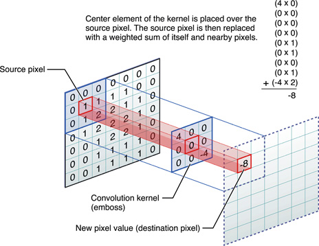
Strictly speaking, convolutional layers are a slight misnomer, since the operations are typically expressed as cross correlations.

After the filters have passed over the image, a feature map is generated for each filter.

Because the kernel has a width greater than one, and we can only computer the cross-correlation for locations where the kernel fits wholly within the image.
若輸入的影像大小為H x W, kernel大小為h x w, 則輸出影像大小為
(H − h + 1)×(W − w + 1)
Convolution是針對整個輸入處理, 每隔一個固定的間隔(pixels)會移動kernel, 由左至右, 由上至下, 直到整個輸入的所有位置都執行過convolution.
在CNN中對輸入資料做Convolution的運算, 就相當於在fully connected layers中輸入資料和權重的乘法運算.
Convolution的輸出也會接著一個bias運算後再接一個activation output.
7.2.3 Padding
If the input is 5 x 5 and a 3 × 3 filter is used, only 3 x 3 source pixels are convoluted and the feature map is a 3 x 3 grid.
This is called the border effect.
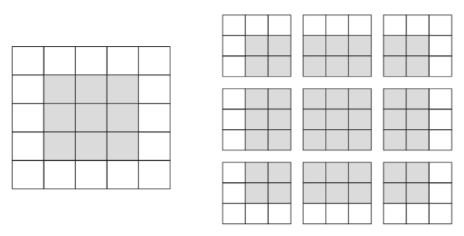
若Convolution輸出的資料會比輸入的資料少, 重覆幾次Convolution過程就會使輸出變成1.
If you want to get an output feature map with the same spatial dimensions as the input, you can use padding.
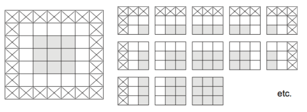
若我們總共加了padding為pH(上和下)列及pW(左跟右)行, 則輸出影像大小為
(H − h + pH + 1)×(W − w + pW + 1)
  pH = h − 1
  pW = w − 1
7.2.4 Stride
When computing the cross-correlation, we start with the convolution window at the top-left corner of the input array, and then slide it over all locations both down and to the right. In previous examples, we default to sliding one pixel at a time. However, sometimes, either for computational efficiency or because we wish to downsampling, we move our window more than one pixel at a time, skipping the intermediate locations.
We refer to the number of rows and columns traversed per slide as the stride.
Cross-correlation with strides of 3 and 2 for height and width respectively:

若stride為sH(高)列及sW(寬)行, 則輸出影像大小為
( (H − h + pH)/sH + 1) × ( (W − w + pW)/sW + 1 )
7.2.5 三維的捲積
If we have many kernels applying to a 2D image, how are these combined in our network to help us get our final result?
Each kernel(filter) generate a 2D feature map, a 3D output is generated for many filters.

7.2.6 以區塊的概念來檢視
若輸入的三維影像資料高為H, 寬為W, 色分量為3
From a data perspective, that means that a single image provided as input to the model is, in fact, three images.
If an input image has 3 channels (e.g. a depth of 3), then a filter applied to that image must also have 3 channels (e.g. a depth of 3).
當使用的filter有F個, convolution後的結果為F x H x W 的三維輸出
Each filter has its own specific filter weights for each of the three channels.
Regardless of the depth of the input, the filter is applied to the input using a dot product operation which results in a single value.

For example, it is common for a convolutional layer to learn from 32 to 512 filters in parallel for a given input.
In a convolutional layer, we are basically applying multiple filters at over the image to extract different features. But most importantly, we are learning those filters!
7.2.7 批次處理
7.3 Pooling層
After obtaining features using convolution, we would next like to use them for classification.
But, this can be computationally challenging.
For ex.,:
- images of size 96 x 96 pixels
- we have learned 400 features with 8x8 kernel
- each filter has a (96−8+1)∗(96−8+1) = 7921 feature map
- each image has 7921 ∗ 400 = 3,168,400 features output
Thus, to describe a large image, one natural approach is to aggregate statistics of these features at various locations.
The Pooling layer is responsible for reducing the spatial size of the Convolved Feature:
- max pooling It takes the maximum value in a certain filter region
- average pooling It takes the average value in a filter region.

Max Pooling會取滑動視窗中的最大值代表這個區域
7.3.1 Pooling層的特徴
- 沒有學習參數 直接從目標區域中取值
- 色層的數量不變 每一個色層分別地進行Pooling
- 因位置引起的微小的變化不改變結果 因為是考慮一個區域 區域內的微小變化幾乎不影響結果
7.4 實作Convolution/Pooling Layers
7.4.1 4維配列
處理影像時, 輸入的資料是四維的陣列:( 樣本數, 色層, 高, 寬 )
操作四維資料的例子:
import numpy as np

x = np.random.rand(10, 1, 28, 28)
x.shape # (10, 1, 28, 28)
x[0].shape # (1, 28, 28)
x[1].shape # (1, 28, 28)
( 色層, 高, 寬 )
It is not easy to write a code for convolution of 4D images and 3D filters.
7.4.2 利用im2col
Matlab提供im2col來把輸入的image block轉成columns
There is a simple method to convolution batch images and multiple filters. The method is usually called im2col in popular machine learning frameworks.
With im2col and matrix reshape, convolution is replaced with dot product.
Assume that:
- input image is (3 ,4 , 4 )
- kernel is ( 3, 2, 2)
- stride = 1
- padding = 0
With img2col,
- each local windowed image is reshaped in to a (4 + 4 + 4) x 1 column and build a 12 x 9 matrix
- kernel is reshaped into a 1 x (2 x 2 x 3) row matrix
- The convolution is basically a dot-product between the kernel filter and the local regions selected by the moving window.


使用img2col的缺點是需要額外的記憶體儲存展開後的影像
7.4.3 Convolution的實作
common/util.py:
def im2col(input_data, filter_h, filter_w, stride=1, pad=0):
    """

    Parameters
    ----------
    input_data : 輸入數據由四維數組組成(數目,通道,高度,寬度)
    filter_h : filter高度
    filter_w : filter weight
    stride :
    pad :

    Returns
    -------
    col : 2次元配列
    """
    N, C, H, W = input_data.shape
    out_h = (H + 2*pad - filter_h)//stride + 1
    out_w = (W + 2*pad - filter_w)//stride + 1
    # only padding the image
    img = np.pad(input_data, [(0,0), (0,0), (pad, pad), (pad, pad)], 'constant')
    col = np.zeros((N, C, filter_h, filter_w, out_h, out_w))

    for y in range(filter_h):
        y_max = y + stride*out_h
        for x in range(filter_w):
            x_max = x + stride*out_w
            col[:, :, y, x, :, :] = img[:, :, y:y_max:stride, x:x_max:stride]

    col = col.transpose(0, 4, 5, 1, 2, 3).reshape(N*out_h*out_w, -1)
    return col

def col2im(col, input_shape, filter_h, filter_w, stride=1, pad=0):
    """

    Parameters
    ----------
    col :
    input_shape : 入力データの形状(例:(10, 1, 28, 28))
    filter_h :
    filter_w
    stride
    pad

    Returns
    -------

    """
    N, C, H, W = input_shape
    out_h = (H + 2*pad - filter_h)//stride + 1
    out_w = (W + 2*pad - filter_w)//stride + 1
    col = col.reshape(N, out_h, out_w, C, filter_h, filter_w).transpose(0, 3, 4, 5, 1, 2)

    img = np.zeros((N, C, H + 2*pad + stride - 1, W + 2*pad + stride - 1))
    for y in range(filter_h):
        y_max = y + stride*out_h
        for x in range(filter_w):
            x_max = x + stride*out_w
            img[:, :, y:y_max:stride, x:x_max:stride] += col[:, :, y, x, :, :]

    return img[:, :, pad:H + pad, pad:W + pad]
- numpy.pad(array, pad_width, mode='constant', **kwargs) Pad an array.
- array The array to pad.
- pad_width Number of values padded to the edges of each axis. ((before_0, after_0), … (before_N, after_N)) unique pad widths for each axis.
- mode
- 'constant’ Pads with a constant value.
a = [0, 1, 2, 3, 4, 5]
np.pad(a, (2, 3), 'constant', constant_values=(8, 9))

array([8, 8, 0, 1, 2, 3, 4, 5, 9, 9, 9])
- Default transpose
- permute the axes
x = np.arange(4).reshape((2,2))
print(x)

array([[0, 1],
       [2, 3]])

np.transpose(x)

array([[0, 2],
       [1, 3]])
x = np.ones((1, 2, 3))
np.transpose(x, (1, 0, 2)).shape

(2, 1, 3)
Test im2col:
- 1 sample of 7 x 7 image using a 5 x 5 kernel
import sys, os
sys.path.append(os.pardir)
from common.util import im2col

x1 = np.random.rand(1,3,7,7)
col1 = im2col(x1, 5, 5, stride=1, pad=0)
print(col1.shape)


# 9  : the number of sliding kernel window
# 75 : the number of pixels covered by each convolution( 25 pixels ) for 3 color depth
(9, 75)
x2 = np.random.rand(10,3,7,7)
col2 = im2col(x1, 5, 5, stride=1, pad=0)
print(col2.shape)


# 90 : the number of sliding kernel window
# 75 : the number of pixels covered by each convolution( 25 pixels ) for 3 color depth
(90, 75)
class Convolution:
    def __init__(self, W, b, stride=1, pad=0):
        # define the number of kernel and kernel size to be used
        self.W = W
        self.b = b
        self.stride = stride
        self.pad = pad

        # (backward時使用)
        self.x = None
        self.col = None
        self.col_W = None

        # gradient
        self.dW = None
        self.db = None

    def forward(self, x):
        # FN: filter number
        # C: color depth
        # FH: filter height
        # FW: filter width
        FN, C, FH, FW = self.W.shape
        N, C, H, W = x.shape
        out_h = 1 + int((H + 2*self.pad - FH) / self.stride)
        out_w = 1 + int((W + 2*self.pad - FW) / self.stride)

        col = im2col(x, FH, FW, self.stride, self.pad)
        # each filter is expanded to be in one row
        col_W = self.W.reshape(FN, -1).T

        # the same dot operation as Affine transform
        out = np.dot(col, col_W) + self.b
        out = out.reshape(N, out_h, out_w, -1).transpose(0, 3, 1, 2)

        self.x = x
        self.col = col
        self.col_W = col_W

        return out

    def backward(self, dout):
        FN, C, FH, FW = self.W.shape
        dout = dout.transpose(0,2,3,1).reshape(-1, FN)

        self.db = np.sum(dout, axis=0)
        self.dW = np.dot(self.col.T, dout)
        self.dW = self.dW.transpose(1, 0).reshape(FN, C, FH, FW)

        dcol = np.dot(dout, self.col_W.T)
        dx = col2im(dcol, self.x.shape, FH, FW, self.stride, self.pad)

        return dx
7.4.4 實作Pooling Layer
The pooling layer, is used to reduce the spatial dimensions, but not depth, on a convolution neural network.
The max-pooling layer, which slides a window, like a normal convolution(except the color depth is processed independntly), and get the biggest value on the window as the output.
class Pooling:
    def __init__(self, pool_h, pool_w, stride=1, pad=0):
        self.pool_h = pool_h
        self.pool_w = pool_w
        self.stride = stride
        self.pad = pad

        self.x = None
        self.arg_max = None

    def forward(self, x):
        N, C, H, W = x.shape
        out_h = int(1 + (H - self.pool_h) / self.stride)
        out_w = int(1 + (W - self.pool_w) / self.stride)

        col = im2col(x, self.pool_h, self.pool_w, self.stride, self.pad)
        col = col.reshape(-1, self.pool_h*self.pool_w)
        # calculate the max. of each row
        arg_max = np.argmax(col, axis=1)
        out = np.max(col, axis=1)
        out = out.reshape(N, out_h, out_w, C).transpose(0, 3, 1, 2)

        self.x = x
        self.arg_max = arg_max

        return out

    def backward(self, dout):
        dout = dout.transpose(0, 2, 3, 1)

        pool_size = self.pool_h * self.pool_w
        dmax = np.zeros((dout.size, pool_size))
        dmax[np.arange(self.arg_max.size), self.arg_max.flatten()] = dout.flatten()
        dmax = dmax.reshape(dout.shape + (pool_size,))

        dcol = dmax.reshape(dmax.shape[0] * dmax.shape[1] * dmax.shape[2], -1)
        dx = col2im(dcol, self.x.shape, self.pool_h, self.pool_w, self.stride, self.pad)

        return dx
- np.argmax() Return an index of the max. value along a axis.
- np.max() Return the max. value along a axis.
7.5 CNN的實作
卷積神經網路(Convolutional Neural Network, CNN)is composed of the following layers:
- Convolution layer Generate a feature map
- ReLU layer(Rectified Linear Units) 它可以增強判定函式和整個神經網路的非線性特性,相比其它函式來說,ReLU函式更受青睞,這是因為它可以將神經網路的訓練速度提升數倍,而並不會對模型的泛化準確度造成顯著影響。
- Pooling layer 池化層會對空間大小down-sampling,因此參數的數量和計算量也會下降,這在一定程度上也控制了over-fitting。通常來說,CNN的卷積層之間都會周期性地插入池化層。
- Loss/Decision layer 決定訓練過程如何來「懲罰」網路的預測結果和真實結果之間的差異,它通常是網路的最後一層。 各種不同的損失函式適用於不同類型的任務。例如,
- Softmax + 交叉熵損失函式 常常被用於在K個類別中選出一個
- Sigmoid交叉熵損失函式 常常用於多個獨立的二分類問題
- 歐幾里德損失函式 常常用於結果取值範圍為任意實數的問題

ch07/train_convnet.py:
import sys, os
sys.path.append(os.pardir)  # 親ディレクトリのファイルをインポートするための設定
import numpy as np
import matplotlib.pyplot as plt
from dataset.mnist import load_mnist
from ch07.simple_convnet import SimpleConvNet
from common.trainer import Trainer

# データの読み込み
(x_train, t_train), (x_test, t_test) = load_mnist(flatten=False)

# 処理に時間のかかる場合はデータを削減
#x_train, t_train = x_train[:5000], t_train[:5000]
#x_test, t_test = x_test[:1000], t_test[:1000]

max_epochs = 20

network = SimpleConvNet(input_dim=(1,28,28),
                        conv_param = {'filter_num': 30, 'filter_size': 5, 'pad': 0, 'stride': 1},
                        hidden_size=100, output_size=10, weight_init_std=0.01)

trainer = Trainer(network, x_train, t_train, x_test, t_test,
                  epochs=max_epochs, mini_batch_size=100,
                  optimizer='Adam', optimizer_param={'lr': 0.001},
                  evaluate_sample_num_per_epoch=1000)
trainer.train()

# パラメータの保存
network.save_params("params.pkl")
print("Saved Network Parameters!")

# グラフの描画
markers = {'train': 'o', 'test': 's'}
x = np.arange(max_epochs)
plt.plot(x, trainer.train_acc_list, marker='o', label='train', markevery=2)
plt.plot(x, trainer.test_acc_list, marker='s', label='test', markevery=2)
plt.xlabel("epochs")
plt.ylabel("accuracy")
plt.ylim(0, 1.0)
plt.legend(loc='lower right')
plt.show()
...
train loss:0.0047506178614996515
=============== Final Test Accuracy ===============
test acc:0.9877
Saved Network Parameters!

7.6 CNN的視覺
7.6.1 第一層的視覺
kernel在學習前與學習後的比較:
import numpy as np
import matplotlib.pyplot as plt
sys.path.append(os.pardir)
from ch07.simple_convnet import SimpleConvNet

def filter_show(filters, nx=8, margin=3, scale=10):
    """
    c.f. https://gist.github.com/aidiary/07d530d5e08011832b12#file-draw_weight-py
    """
    FN, C, FH, FW = filters.shape
    ny = int(np.ceil(FN / nx))

    fig = plt.figure()
    fig.subplots_adjust(left=0, right=1, bottom=0, top=1, hspace=0.05, wspace=0.05)

    for i in range(FN):
        ax = fig.add_subplot(ny, nx, i+1, xticks=[], yticks=[])
        ax.imshow(filters[i, 0], cmap=plt.cm.gray_r, interpolation='nearest')
    plt.show()


network = SimpleConvNet()
# ランダム初期化後の重み
filter_show(network.params['W1'])

# 学習後の重み
network.load_params("params.pkl")
filter_show(network.params['W1'])
- 學習前
- 學習後


7.6.2 通過層次結構擷取信息
7.7 代表性的CNN
7.7.1 LeNet
INPUT => CONV => RELU => POOL => CONV => RELU => POOL => FC => RELU => FC
LeNet與現在CNN的作法差異
- sigmoid vs. ReLU
- sub-sampling vs. max pooling
7.7.2 AlexNet
AlexNet與LeNet的作法差異
- sigmoid vs. ReLU
- 使用Local Response Normalization
- 使用Droupout
8 深度學習
深度學習是加深層數後的多層神經網路
多層神經網路有必須要考慮的問題
8.1 更深的網絡
8.1.1 更多層的網絡
8.1.2 さらに認識精度を高めるには
8.1.3 層を深くすることのモチベーション
8.2 ディープラーニングの小歴史
8.2.1 ImageNet
8.2.2 VGG
8.2.3 GoogLeNet
8.2.4 ResNet
8.3 ディープラーニングの高速化
8.3.1 取り組むべき問題
8.3.2 GPUによる高速化
8.3.3 分散学習
8.3.4 演算精度のビット削減
8.4 ディープラーニングの実用例
8.4.1 物体検出
8.4.2 セグメンテーション
8.4.3 画像キャプション生成
8.5 ディープラーニングの未来
8.5.1 画像スタイル変換
8.5.2 画像生成
8.5.3 自動運転
8.5.4 Deep Q-Network(強化学習)
8.6 まとめ
A Softmax-with-Lossレイヤの計算グラフA.1 順伝播
A.2 逆伝播
A.3 まとめ
AI Deep Learning .net

留言